Using contrast agents to obtain maps of regional perfusion and capillary wall permeability

Ronnie Wirestam^*

Department of Medical Radiation Physics, Lund University, University Hospital, SE-221 85 Lund, Sweden

*Corresponding Author:

Fax: +46 4617 8540
Email: ronnie.wirestam@med.lu.se

Abstract

Tracer kinetic modeling for quantification of perfusion and capillary wall permeability is a well-established approach, applied to various imaging modalities. In this review, methods employing intravascular as well as diffusible nonradioactive contrast agents for characterization of tissue microcirculation and microvasculature are described. The article focuses on perfusion and permeability imaging by MRI, particularly for brain applications, and the use of alternative medical imaging methods, such as CT and ultrasound, is also briefly introduced.

Keywords

capillary wall permeability; contrast agent; dynamic studies; medical imaging; perfusion; tissue blood flow; tracer kinetics

The term perfusion imaging refers, traditionally, to the use of a medical imaging modality for measurements of tissue capillary blood flow [1], although it has become increasingly common to include other characteristics of tissue microcirculation and microvasculature in the perfusion imaging framework. In quantitative approaches, the regional perfusion is normally visualized as a parametric map calculated on the basis of an appropriate tracer-kinetic model. Perfusion imaging is of obvious importance for assessment of cerebral blood flow (CBF) and myocardial blood flow, although investigations of numerous other organs or tissue types are also highly relevant. Quantitative or semi-quantitative estimates of perfusion or regional blood flow can serve as important markers of tissue function and viability. Brain perfusion imaging has found applications in ischemic stroke, dementia and trauma, among others. Perfusion imaging in oncology is used extensively throughout the body [2], often in combination with assessment of capillary wall permeability, and extracted parameters are applied to tumor characterization and grading [3], as well as in the assessment of pharmacological efficiency and follow-up and outcome of treatment [4].

Perfusion measurements using radioisotopes have been available for many years, using SPECT and PET. Stable xenon-CT is another reference method for CBF measurements. This article is primarily dedicated to perfusion and permeability imaging by using non-radioactive contrast agents (CAs), developed for general diagnostic use in combination with an appropriate medical imaging technique in a clinical environment. It should be noted that the term ‘indicator’ would, formally, be a better choice of terminology than ‘tracer’ for such substances, since a tracer is, in the classic literature, defined as an indicator molecule that is identical to (and thereby ‘traces’) the corresponding systemic carrier substance [5]. However, it has always been very common not to firmly distinguish between the two terms. This overview will primarily focus on MRI methods, but the application of similar concepts to CT and ultrasound (US) will also be briefly introduced. CT offers excellent availability also in the acute setting, and US has the additional advantage of being portable as well as readily available. MRI offers the combined advantages of quite reasonable availability and the possibility to obtain additional information about softtissue morphology, diffusion, large vessels and metabolism during a single imaging session.

Tracers & the microcirculation: basic considerations

The microvasculature is characterized by exchange of fluid, oxygen, nutrients, hormones and anti-infective agents between blood and surrounding tissue, and also by removal of carbon dioxide and other waste products. Large variations are seen in the geometry and topography of the microvascular beds between different types of tissue [6]. In the microvasculature, the blood flow is determined by the balance between viscous stresses and pressure gradients. Arterioles have a coat dominated by smooth muscle, capable of large resistance to blood flow, while venular muscular coating is generally sparser. Capillaries, with diameters of the order of 10 μm, lack muscular coat and connect arterioles and venules. Due to the high arteriolar resistance, the pressure in the capillaries is fairly independent of the arterial pressure. There is, however, not much resistance between capillaries and veins, so the venous pressure has considerable effect on the capillary pressure. The smooth muscle of the microcirculation acts to regulate the blood flow locally. It is a striking feature of the capillary network to be able to maintain a steady output flow in spite of arterial pulsations, but also to continuously vary the blood flow in order to deliver appropriate amounts of oxygen and nutrients in response to the specific metabolic demand of the cells. Local control of blood flow in the body is achieved by several means [7]. Autoregulation is one such process, explained by myogenic and metabolic mechanisms, normally described as the intrinsic ability of an organ to maintain a constant level of blood flow despite changes in the perfusion pressure. Most systems of the body exhibit some degree of autoregulation, but it is most pronounced in the kidney, heart and brain.

The capillaries of the brain require some special attention. All blood vessels have a smooth inside layer of endothelial cells, but for cerebral capillaries the vascular endothelium constitutes a barrier preventing the passage of large molecules, the so-called blood–brain barrier (BBB). The BBB, and its state of integrity, is important in cerebral perfusion quantification because certain common CAs can act as intravascular tracers (i.e., being nondiffusible from the intravascular to the extravascular space) in measurements of brain perfusion, while being diffusible or partially diffusible from the intravascular to the extravascular space when applied to noncerebral tissue. Furthermore, a diffusible tracer (e.g., labeled water) is typically not freely diffusible in the brain, and its permeability or degree of extraction must be considered in the perfusion quantification.

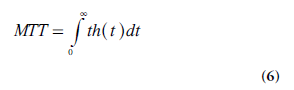
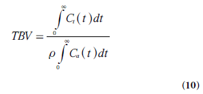
A number of physiologically relevant parameters, specific to the employed methodology and type of tracer or indicator, can be extracted by kinetic modeling to describe the hemodynamics and permeability of the microvasculature. The term perfusion refers to the flow of blood through the capillary system. Perfusion or tissue blood flow (TBF) is traditionally quantified in terms of the volume of blood transported to a given mass (or volume) of tissue per unit time, typically in units of ml/min/100 g (or ml/min/100 ml). Other microvascular characteristics are sometimes loosely included in the term ‘perfusion parameters’, for example, the mean transit time (MTT; in seconds), which is the average time it takes for the blood (or plasma) to travel through the capillary network from the arterial to the venous end, and the tissue blood volume (TBV; ml/100 g or ml/100 ml). Additionally, a number of non- or semi-quantitative perfusion indices have been proposed in various applications. Below, TBV refers to the volume of whole blood per unit mass of tissue and, similarly, TBF refers to the flow of whole blood per unit mass of tissue.

The relationship between blood flow, blood volume and blood mean transit time is given by the central volume theorem [8]:

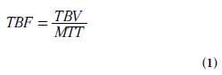
Particularly in cerebral applications, it can be useful to have access to information about blood volume and/or mean transit time, in addition to blood flow, because combined data may facilitate assessment of whether autoregulation mechanisms are engaged to maintain the local blood flow under circumstances with altered perfusion pressure. Furthermore, the blood volume parameter may contribute to identification of regions with angiogenesis/neovascularization.

One of the most basic considerations in tracerkinetic theory is the concept of mass balance, introduced by the so-called Fick principle [9]:

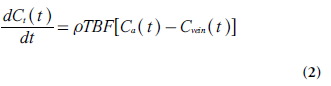
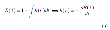
Where C_t(t), C_a(t) and C_vein(t) are the tracer concentrations (M), as a function of time t, in the tissue element, in the tissue-supplying artery (arterial inlet) and in the vein of outflow (venous outlet), respectively, and ρ is tissue density. Different tracer molecules exhibit different transit times when passing through the system, and the function h(t) describes the distribution (frequency function) of transit times (following an instantaneous input of tracer molecules at t = 0). Another basic parameter is the tissue residue function R(t) [10], defined as the fraction of tracer molecules still remaining in the tissue of interest at time t, after having entered the tissue at time t = 0. Obviously, R (0) = 1 and the residue function shows a monotonic decrease with time. R(t) is related to h(t) according to the following relationship:

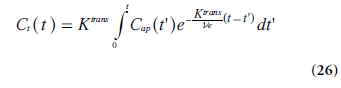
An important and general relationship between TBF, C_t(t) and C_a(t), for stationary and linear systems, is the convolution integral [10]. The amount of tracer molecules (in moles) that enters the tissue volume of interest V_t(with mass ρV_t) between time t and t + dt is given by the product TBF Ca(t) rVt dt. From the definition of the tissue residue function, it is clear that, at times t >t, this amount of tracer contributes by R(t-t) TBF Ca (t) rV_t dτ to the total amount of tracer molecules in the tissue volume. Integration over all entrance times t from 0 to t gives the total amount of tracer molecules in the tissue volume at time t. Finally, division by the tissue volume V_tprovides the tissue concentration C_t:

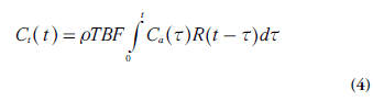
Which by definition constitutes a convolution integral. It is of some relevance to note that the indicator dilution theory leading to Equation 4 makes no specific assumptions about the internal tissue architecture or the tracer transport mechanisms within the tissue volume.

In this context, it is also appropriate to introduce the tissue impulse response function Q_t, which is a frequently used concept to characterize the system and the employed tracer:

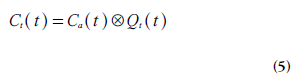
Where denotes convolution. Retrieval of the tissue impulse response function from measured tracer concentration data is typically achieved either by model-independent deconvolution or by an analytical description of Q_t(t) based on compartmental modeling. Examples of such data analysis methods will be further described below, but it should already at this point be emphasized that the interpretation of the impulse response function is dependent on the specific approach used, as described in detail by Brix et al. [11]. When model-independent deconvolution is applied in combination with the general indicator dilution theory [10], it is clear from Equations 4 & 5 that Q_t(t) = rTBF R(t) and Q_t(0) = rTBF. However, when data analysis is carried out by compartment modeling, Q_t(0) has other (model-specific) properties and is, in general, not expected to represent perfusion. Both these data analysis strategies are associated with pitfalls, and the interpretation of obtained parameters is not always straightforward [11].

In the following sections, the basic concepts of perfusion quantification are put into the context of medical imaging with the tracer or indicator being a conventional clinical CA (e.g., Gd-chelates in MRI and iodinated substances in CT). Such CAs are typically extracellular (i.e., while in the vascular compartment the tracer molecules reside in the blood plasma volume and upon extraction from the blood pool, if applicable, they distribute into the extravascular, extracellular space [EES]). In the description below, adaptations to the use of an extracellular tracer are generally indicated. Application of accurate values of blood hematocrit (Hct) can thus be of practical relevance in certain cases. It should be noted that the hematocrit is approximately 0.45 for major vessels and considerably lower (~0.25) in small vessels (capillaries). Unless explicit distinction between hematocrit in large and small vessels is required, the general notation Hct is used below to represent the hematocrit of the actual blood vessel size in question.

Intravascular tracers

Applications of the theory of intravascular or nondiffusible tracers [10,12] are exemplified by dynamic susceptibility contrast (DSC)-MRI and dynamic perfusion CT for measurement of cerebral perfusion parameters, primarily CBF, cerebral blood volume (CBV) and blood MTT. The CA is administered intravenously during a relatively short injection time (at injection rates of the order of 5 ml/s), referred to as a bolus injection. During the subsequent passage through the circulatory system the bolus is further broadened, and, in practice, the arterial tracer arrives at the local capillary system during an extended time period, and the shape of the bolus upon arrival is described by the arterial input function (AIF), that is, the arterial CA concentration curve C_a(t).

In this context, the MTT is the average time it takes for an intravascular tracer (representing blood or plasma) to pass through a microvascular or capillary system from the arterial to the venous side. MTT is defined as the expectation value of the transit time distribution h(t) – that is:

Using the derivative h(t) = −dR(t)/dt (Equation 3) in an integration by parts of the function 1-R(t), the following relationship is obtained:

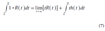
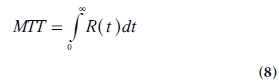
Meier and Zierler demonstrated that, for a finite volume, [tR(t)]→0 when t→∞ [12], and MTT is thus given by:

A useful expression for calculation of TBV (i.e., the capillary volume per unit mass of tissue) can be derived using the convolution integral (Equation 4) in combination with the central volume theorem (Equation 1) and the relationship between MTT and R(t) (Equation 8). It follows from Fubini’s theorem that the integral, over the whole space, of the convolution of two functions is given by the product of their respective integrals. Hence, integration of C_t(t) from zero to infinity can, according to Equations 4 & 5, be expressed as follows:

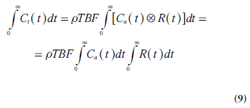
By replacing TBF in Equation 9 by a combination of Equations 1 & 8 and solving for TBV, the following relationship is obtained:

In cerebral bolus-tracking applications, using the notation AIF(t) for the arterial concentration curve of the CA bolus, CBV can be expressed as follows, including adaptation to the use of a plasma tracer (and different hematocrit levels in arteries and capillaries):

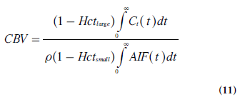
where Hct_largeand Hct_smallare the hematocrit values in large and small vessels, respectively.

After appropriate corrections for the use of a plasma tracer, the measured tissue concentration curve C_t(t) is given by the convolution of a kernel, that is, the impulse response function ρCBF R(t), and the AIF (Equations 4–5) [10,13,14]:

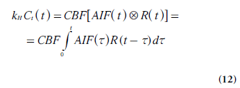
Where denotes convolution and k_H = [1- Hct_large ]/[ρ(1 - Hct_small)], in analogy with the CBV case above [13]. By independently acquiring Ct(t) from the tissue of interest and the AIF from a suitable tissue-feeding artery, CBF can thus be determined from the maximal value of the tissue impulse response function obtained by model-free deconvolution.

In practice, MTT is often acquired from the CBV:CBF ratio (using Equations 11 & 12), according to the central volume theorem (Equation 1). Obviously, MTT can also be calculated from the output of the deconvolution using Equation 8, which is sometimes reformulated according to Zierler’s area:height relationship [15]:

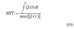
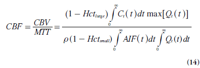
An alternative formulation of CBF is thus given by Equation 14 [13,16]. It follows directly from the properties of R(t) that the expression in Equation 14 is equivalent to rCBF = max[Q_t(t)] = max[r CBF R(t)], as stated above.

Finally, the required deconvolution is, in general, a delicate mathematical procedure, especially in the presence of noise. A number of model-dependent [17] and model-free [18,19] deconvolution algorithms have been proposed, as well as deconvolution using statistical approaches [20,21]. However, model-free matrix formulation of the convolution integral solved by means of singular value decomposition (preferably the blockcirculant version) has been the most frequently applied approach in DSC-MRI [22].

Use of intravascular tracers in medical imaging

MRI

DSC-MRI is frequently used for assessment of cerebral perfusion [13,19,23]. After rapid intravenous injection of the CA bolus, followed by a saline flush, the first passage of CA through the brain vasculature is monitored by T2*-weighted MRI. In combination with kinetic models for intravascular tracers, as described above, this enables calculation of CBF, CBV and MTT maps (Figure 1).

In DSC-MRI examinations, a conventional paramagnetic gadolinium-based CA is normally used, assumed to act as an intravascular tracer in the presence of an intact BBB. Several studies have been carried out on the use of gadolinium chelates at different doses and preparations [24–27], as well as on the effects of sequential administrations of CA [28]. Preparations with a high gadolinium concentration (1 M) have been developed, enabling a higher dose to be administered in a given volume of injection [24]. The use of gadolinium-based CAs in MRI is generally very safe, although anaphylactoid reactions (at very low incidence rates) have been reported, as well as a severe but extremely rare complication referred to as nephrogenic systemic fibrosis, observed in patients with renal impairment (predominantly after receiving more than a normal dose of gadolinium CA) [29].

During its passage through the brain, the exogenous paramagnetic CA causes transient local magnetic field gradients that extend from the vascular compartment into the surrounding tissue (although the CA itself is assumed not to leave the blood pool). These local CA-induced magnetic field inhomogeneities introduce a phase dispersion of the water proton spins, and a corresponding signal drop in T₂^*-weighted images during the bolus passage [30]. Gradientecho- based pulse sequences, not refocusing the spin dephasing caused by magnetic field inhomogeneities, are frequently used for this purpose, but spin-echo sequences exhibit substantial signal loss as well in a DSC-MRI experiment due to spin diffusion in the CA-induced magnetic field gradients in combination with T₂ shortening within the vascular compartment.

The choice between gradient-echo and spinecho sequences has been a somewhat controversial issue in DSC-MRI. Gradient echoes typically show a higher sensitivity to a given dose of CA, that is, a larger relative signal drop at peak concentration and higher contrast-to-noise ratio. However, early simulations predicted that the spin-echo signal would be selectively more sensitive to CA residing in the microvasculature (vessels with diameters of the order of 5–10 μm) [31], and this finding was supported by experimental studies [32,33]. Still, investigations comparing gradient-echo and spin-echo sequences with regard to clinical usefulness have not been entirely conclusive [32,34]. In brief, gradientecho sequences tend to show more susceptibility artefacts and large-vessel hyperintensity in CBV and CBF maps (Figure 2B), while spin echoes may require higher CA dose to achieve sufficient signal drop at peak concentration (at least at lower magnetic field strengths). As will be further discussed below, the T2* relaxivity may depend on the topography of the vascular space in which the intravascular CA is located [35,36], and the behaviour of ΔR₂^*-versus-concentration (C) relationships in blood and tissue environments may also vary between gradient echoes and spin echoes [35]. Recently, a combined spin-echo and gradient-echo sequence was proposed, allowing for T1-insensitive signal collection and enabling vessel-size imaging [37]. With regard to the readout technique in DSC-MRI, single-shot echo-planar imaging (EPI; either gradient echo or spin echo) has been the most common for monitoring the tissue (Figure 2C) and arterial signal-versus-time curves. The primary reason for its popularity is excellent temporal resolution in combination with whole-brain coverage. An alternative approach is to use ‘principles of echo shifting with a train of observations’ (PRESTO), which covers large regions with very short repetition times (TRs) [38].

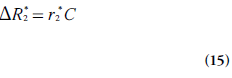
For quantification of CA concentration, C is often approximated to be proportional to the change in transverse relaxation rate ΔR₂^* (with a generally unknown proportionality constant, corresponding to the T₂^* relaxivity, denoted by R₂^*):

For gradient echo-based pulse sequences, being heavily T₂^*-weighted, the signal development over time t, S(t), during the CA passage is given by:

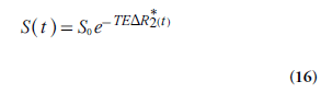
Where S₀ is the baseline signal and TE is echo time. For spin-echo sequences, analogous equations can be formulated for the relationship between signal and the change in the transverse relaxation rate ΔR₂. Note that there is a certain risk of competing T₁ effects in the signal registration, not accounted for in Equation 16 [39].

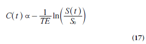
From Equations 15 and 16, the concentration C of the CA (in arbitrary units) can be calculated as:

The situation above is complicated by the fact that the change in the transverse relaxation rate (Equation 15), at a given concentration, depends on the vessel size and the vascular topography [35,40], with substantially higher r₂^* in tissue environments as compared with the arteries used for AIF registration. If this is not accounted for, the resulting AIF area underestimation hampers accurate perfusion quantification in absolute terms, and is probably an important contribution to overestimations of DSC-MRI-based CBV and CBF, observed in experimental comparisons with gold-standard techniques [41–43]. The T₂^* relaxivity issue is made even more difficult by observations of a quadratic ΔR₂^*-versus-C relationship in oxygenated whole blood [44]. This implies that the application of Equation 15 to AIF data acquired from a whole-blood compartment might lead to incorrect AIF shape, and a quadratic model accounting for hematocrit and relaxivity might be more appropriate [45]. Another approach to accomplish a linear CA response, giving a correct gradient echo-based AIF shape, is to select the AIF from pixels at specific locations outside large vessels with appropriate orientation relative the main magnetic field [46]. Phase-based AIFs are also promising in this respect [44,47].

A few additional methodological complications leading to imperfect AIF registration will be briefly discussed (Figure 3). First, it should be noted that the CA concentrations in large vessels are much higher than in tissue, and an echo time (TE) that is reasonably well optimized for tissue regions is likely to cause a decrease of arterial signal to the noise level (sometimes referred to as signal saturation or signal clipping) at peak concentration [48]. Attempts have been made to employ a shorter TE for the slice targeting a brain-feeding artery, while at the same time using a longer TE for brain-tissue slices [49]. Another commonly observed effect is local geometric distortion at peak concentration, such that arterial signal becomes displaced in the image during the bolus passage, owing to the low bandwidth in single-shot EPI [50], and this can be reduced by employing higher-bandwidth pulse sequences such as segmented EPI. Furthermore, partial volume effects in AIF registration are very complex in DSC-MRI, and have received considerable attention [51,52]. Finally, the measured AIF may not accurately represent the artery that actually supplies the tissue of interest. If arterial dispersion (bolus broadening) occurs between the site of registration and the location of the true arterial input, CBF and MTT estimates may be incorrect due to deconvolution with an erroneously shaped AIF (typically being too narrow) [53]. Effects of arterial dispersion can potentially be reduced by employing local arterial input functions [54] or by accounting for dispersion effects in the deconvolution procedure [21,55].

If the BBB is damaged, as commonly observed, for example, in tumor environments, the gadolinium chelate will enter the EES. The assumptions of an intravascular tracer are then violated, and appropriate corrections are likely to be beneficial, in particular for CBV assessment [56]. T₁ signal enhancement, caused by CA in the EES, can also be minimized by administration of a small pre-bolus of CA [57]. The pre-bolus CA is then assumed to result in an almost complete regrowth of longitudinal magnetization between two excitation pulses, thereby eliminating the influence of further shortening of T₁ when the main bolus arrives.

Deconvolution-based approaches for retrieval of perfusion parameters should theoretically not require correction for recirculation (i.e., for CA passing through the tissue of interest multiple times with the circulating blood). However, it has been argued that removal of recirculation effects is likely to be of relevance in DSC-MRI owing to the complex T₂^* relaxivity situation [58], and a common approach has been to fit a γ-variate function to concentration–time data before calculating the perfusion parameters.

Finally, although DSC-MRI-based perfusion estimates tend to show reasonable linear correlation with reference methods, as well as convincing relative CBV and CBF distributions, it is clear that DSC-MRI estimates have generally been overestimated in absolute terms [42,43], most likely due to the sources of AIF-area underestimation described above. A viable solution to this would be to calibrate the DSC-MRI estimates, either by using a general calibration factor obtained from direct comparison with a gold-standard method [41,59], or by acquiring an additional, subject-specific and independent local or global CBV or CBF estimate, for example, a steady-state T₁-based estimate of the CBV [60], for rescaling the absolute level of the DSC-MRI estimates.

CT

Following the initial idea of employing dynamic CT scans enhanced by an iodinated CA for assessment of perfusion by Axel [61], later refinement and adaptation to clinical environments [14,62,63] has led to a powerful tool for perfusion imaging with excellent availability, for example, in connection with acute stroke (where unenhanced CT has been the method of choice for visualization of intracranial hemorrhage for a long time). Today, quantification of CBF, CBV and MTT by dynamic contrast-enhanced CT (Figure 4) employs the bolus-tracking theory of intravascular tracers (including the deconvolution approach), and follows, in principle, the same processing methodology as for DSC-MRI [63]. In perfusion CT, it is also very common to include registration of a venous output function from the superior sagittal sinus to allow for correction of arterial partial volume effects by rescaling the AIF time integral (i.e., the AIF area under curve). This approach is less common in DSC-MRI, although similar concepts have been proposed [43].

From the perspective of CBV and CBF quantification in absolute terms, the most prominent advantage of perfusion CT, compared with DSC-MRI, is the direct and linear relationship between CA concentration and radiodensity. Other quantification issues related to, for example, arterial dispersion and deconvolution of noisy data are, however, of similar concern for both modalities. In practical implementations, perfusion CT protocols typically show excellent spatial resolution, but tended for some time to exhibit reduced brain coverage compared with DSC-MRI. This situation has, however, considerably improved with the continuous development of multiple detector row scanners. Obviously, absorbed dose must be kept to a minimum and settings of low kilovolt and milliampere (80 kVp and 100–120 mA, respectively) have been recommended [63]. Modern iodinated CAs are safe, although uncommon adverse effects exist, primarily anaphylactoid reactions and contrast-induced nephropathy [64].

Noise is an issue in dynamic perfusion CT, and various filtering approaches are normally included in the processing. Accuracy and precision may become influenced by noise, particularly under low perfusion conditions when the change in radiodensity relative baseline is small. In order to illustrate typical contrast-to-noise conditions in dynamic perfusion CT, a concentration-versustime curve from one pixel in normal gray matter, with comparatively high blood flow and volume, is displayed in Figure 5 (see Figure 2, in which similar data for DSC-MRI are shown).

Ultrasound

Dynamic contrast-enhanced US for assessment of perfusion is a promising and rapidly emerging technique [65–67], although, at this point, the concept is not quite as widespread as perfusion CT or DSC-MRI. US CAs consist of gas microbubbles (~1–10 μm in diameter) stabilized by different kinds of shells. The current temporal stability of the microbubbles in combination with appropriate size and intravascular distribution imply that they can act as an intravascular or blood-pool tracer. Clinical US CAs are generally well tolerated, and serious side effects are rarely observed. However, as for all other CAs used in medicine, adverse events can occur (primarily anaphylactoid or vasovagal reactions) [68].

The perfusion quantification approaches are still under development, but extraction of semiquantitative measures from time–intensity curves (Figure 6A) as well as transit times (from arterial input to venous output of CA) following intravenous bolus injection of CA, is presently used for assessment of microcirculation and tumor vascularity in a number of locations in the body. Recently, a deconvolution approach was introduced for assessment of the impact of the arterial input on perfusion parameters measured by dynamic contrast-enhanced US after bolus injection of CA [69].

A refined contrast-enhanced US method for analysis of regional tissue perfusion is to analyze the replenishment kinetics of microbubbles [70], after destruction of an initial steady-state population of microbubbles by high-intensity US (i.e., US with high mechanical index [MI]). After complete destruction of the initial microbubble population, new microbubbles will enter with inflowing blood and the microbubble refill rate in the volume of interest is registered by low MI US transmission and the obtained refill curve is analyzed (Figure 6B). The refill signal curve S_r(t) can, for example, be described by S_r(t) = a(1 - exp(-βt)), and the slope β and the plateau of acoustic intensity a can be used for characterization of the tissue blood flow.

Diffusible tracers

This section primarily describes dynamic imaging following intravenous injection of a partially diffusible tracer, for example, when a common clinical (normally extracellular) CA is used for studies of noncerebral tissue or to conditions when BBB leakage occurs (e.g., in tumor environments). Under these circumstances, a certain fraction of the tracer is expected to be extracted from the intravascular to the extravascular space. The diffusive transcapillary flux of tracer depends on the permeability (in cm/min) and the surface area per unit mass of tissue (in cm²/g), often expressed in terms of a combined quantity referred to as the permeability- surface area product of the capillary wall PS (in ml/min/g). The extraction ratio (or extraction fraction) E is the fraction of inflowing tracer that extravasates during one single capillary transit. After mixing, the tracer is distributed within a volume that is larger than the plasma volume. This so-called volume of distribution V_d is normally expressed in terms of an equivalent volume in relation to a reference fluid. A common approximation for obtaining the extraction ratio, assuming that the capillary bed is modeled as a plug-flow system [71], is given by the Crone–Renkin expression [72,73]:

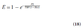
For an extracellular tracer, the leakage originates from the plasma volume, implying the use of plasma flow TBF(1 – Hct) in Equation 18.

This category of studies typically includes a combined assessment of perfusion and permeability, and the pragmatic aim is not always to assess TBF as an isolated parameter. Early MRI studies of the CA transfer coefficient were conducted by Larsson et al. [74], Tofts and Kermode [75], and Brix et al. [76]. It should, at this point, be noted that a variety of physiologic parameters have been introduced in this field of research, and, in many cases, equivalent quantities have been assigned different names and symbols in different studies, and equal or very similar quantities have been difficult to compare because they have been expressed in different units. In this section, the nomenclature of the consensus document by Tofts et al. has been adopted [77].

Standard compartment models

Normally, curve-fitting approaches are employed to extract relevant parameters from experimental data, and more complex models, including a larger number of unknown parameters, tend to generate less reliable estimates. Hence, a pharmacokinetic model presented for use in the context of medical imaging must have reasonable simplicity while still showing a good fit to experimental data. For example, the two-compartment exchange model is defined by [71]:

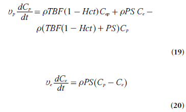
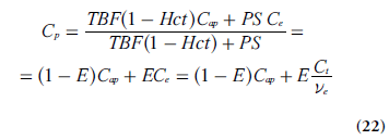
where C_ap is the tracer concentration in the arterial plasma (arterial inlet; M), C_p is tracer concentration in blood plasma (M), C_e is the EES concentration (M), v_p is the fractional plasma volume and ve is the fractional EES volume. If the effect of tracer in the intravascular space is assumed to be negligible, in other words, if the blood volume is small (v_p ≈ 0), then Ct = veCe and dC_t/d_t = v_e(dC_e/d_t).

Mixed flow-permeability weighting: tracer uptake influenced by both flow & permeability

Using the steady-state plasma concentrations at the arterial inlet (C_ap) and the venous outlet (C_v), without tracer backflux from the interstitial space to plasma (i.e.,ρ PS C_e= 0), the extraction ratio E is defined by E = (C_ap-C_v)/C_ap. Sourbron and Buckley [71] introduced a formulation of E when the capillary bed is a compartment (with Cv = Cp by definition), using the fact that, at steady-state, dCp/dt = 0. Under the above conditions,

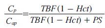
(according to Equation 19) and the extraction ratio of the plasma compartment is thus given by:

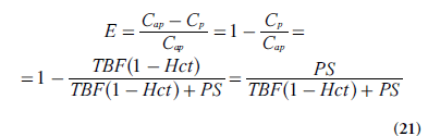
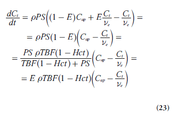
With negligible intravascular tracer (v_p = 0 and C_e = C_t/v_e), combination of Equations 19 & 21 leads to:

Insertion of Equation 22 into Equation 20 (using dC_t /d_t = v_e(dC_e /d_t) gives:

Tofts model & extended version

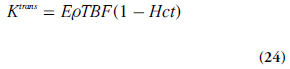
One common approach has been to include the effects of several physiological properties into one composite model parameter, for example, the volume transfer constant between blood plasma and EES, K_trans (s^-1):

Using this notation, the tracer uptake rate in tissue (per unit volume of tissue) can be expressed as:

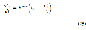
It is also illustrative to briefly address two special cases, which can be evaluated using Equations 21 & 24. At high permeability, when the transcapillary transport is limited by blood flow (PS>>TBF(1 – Hct)), then Ktrans represents the plasma blood flow (i.e., Ktrans ≈ rTBF(1 – Hct)). In the other limiting case, when low capillary permeability limits the tracer leakage (PS<<TBF(1-Hct)), then K^trans reflects the permeability– surface area product (PS), that is, K^trans ≈ ρPS. Note, however, that the case of PS = 0 is not compatible with a Tofts model [71].

The differential equation in Equation 25 has the following solution (if C_ap(0) = C_t (0) = 0):

The approach described above is compatible with the model proposed by Kety [78], and it closely reflects the work by Tofts and Kermode [75] and Larsson et al. [74]. The measured dynamic change in tissue concentration can be viewed upon as a convolution of an exponential kernel and an arterial blood or plasma concentration curve (i.e., the AIF). The notation K^trans was introduced to accentuate that PS and TBF(1 - Hct) cannot be measured separately in tissue environments where the Tofts model is applicable. Brix et al. [76]. introduced a similar methodology, but included the plasma concentration as an additional free model parameter. When the blood volume cannot be assumed to be small, a modified or extended Tofts model is often applied [79], including C_ap(t) and the fractional plasma volume v_p in an additional term:

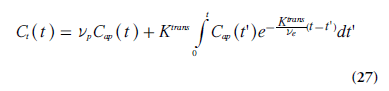
A detailed analysis of the scope and interpretation of the Tofts and extended Tofts models in dynamic contrast-enhanced (DCE)-MRI is given by Sourbron and Buckley [71].

Distributed parameter models

The Tofts–Kermode concept yields K^trans and v_e (and v_p in the extended model), but, as pointed out above, Ktrans does not allow for a separate estimation of blood flow TBF. It might be tempting, under certain circumstances, to presume that K_trans reflects either permeability or flow, but such a conclusion would be quite dubious without a priori information. There is an obvious interest in extracting estimates of TBF and PS separately, and the employment of distributed parameter models, requiring no assumption of the tracer being instantaneously well mixed in each compartment, is a promising alternative, provided that experimental data of adequate quality can be attained. The tissue homogeneity model [80] is a relatively simple example, and the adiabatic approximation to the tissue homogeneity (AATH) model [81] is one common implementation, requiring the assumption that the tracer concentration changes slowly in the EES compared with the rate of change in the vascular compartment, which is motivated by the fact that the volume of the EES is much larger than the blood plasma volume.

In the context of distributed parameter models, the finite transit time of the tracer through the microvasculature (of the order of seconds) becomes central. During this relatively short period, the entire amount of tracer that entered at the arterial end remains in the total tissue space (including plasma and EES). A fraction E of the tracer is extracted into the EES during the transit-time phase, and the remaining fraction (1-E) exits into the venules after completed transit through the capillary network. Hence, the plasma tracer concentration C_pis dependent on position as well as time, in the sense that Cp varies along the vascular tree while dynamic changes in concentration occur. If capillaries are randomly oriented and in reasonable vicinity of each other, the EES CA can be assumed to be well mixed and its concentration C_e is therefore only dependent on time. The initial vascular phase, during which the capillaries are filled with tracer (and during which a fraction might be extracted into the EES), allows for estimation of the MTT, which in turn allows for derivation of TBF since plasma-volume information is also attainable. The later phase gives Ktrans, and the separate estimates of TBF and Ktrans provides PS using the Crone–Renkin relationship (Equation 18). It is generally acknowledged that the AATH model requires input data of high quality, and, in particular, measurements with high temporal resolution, sufficient to sample the vascular phase, are required [82]. That is, the time between subsequent images must be considerably shorter than the MTT, which is of the order of 4–6 s in the normal brain, but might be several times longer, for example, in certain tumors.

Model-independent deconvolution approach for blood flow estimation

According to the general indicator dilution theory [10], TBF can be estimated by solving the basic tracer kinetic equation (Equation 4) using model-independent deconvolution. As pointed out above, estimation of TBF using the modelfree approach does not require detailed information about the tracer distribution within different compartments, but C_a(t) and C_t(t) must be determined with high temporal resolution (of the order of 1–2 s) during the first passage of the tracer bolus. The central volume theorem applies, but in the presence of leakage, it is obvious that the volume of distribution Vd becomes larger than the plasma volume and the mean residence time of the tracer can be very long in comparison with the blood mean transit time.

Use of partially diffusible tracers in medical imaging

MRI

In T₁-weighted DCE-MRI, the in vivo kinetics of a clinical gadolinium-based MRI CA is monitored, and the DCE-MRI experiment allows for some degree of tracer extravasation into the EES. Although different injection schemes may be used, fast bolus injections into a peripheral vein, followed by a saline flush, is likely to be the most frequent approach nowadays. The dynamic CA-induced shortening of relaxation times alters the MRI signal in a complex manner, described by the pulse-sequence-specific signal equation. In early studies, spin-echo pulse sequences were often used, but due to poor temporal resolution they have largely been replaced by, for example, fast low-angle shot (FLASH), Turbo-FLASH and EPI sequences. A presently widespread choice for the dynamic imaging is a gradient-echo sequence with spoiling of the transverse magnetization (SPGR), described by the following signal equation:

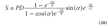
Where PD is proton density and a is flip angle. If changes in T₂^* during the dynamic time series can be neglected, as is often the case at short TE, then the CA can be assumed to influence the signal by its effect on T₁ only. This type of pulse sequence exhibits reasonable, although somewhat limited, spatial coverage, high temporal and spatial resolution as well as sufficient signal-to-noise ratio. The optimal image parameter settings depend strongly on the application and its particular requirements, and it is thus difficult to make distinct recommendations. Flip angles in the range 10–35° and TRs between 2.5 and 8.0 ms were reported in a recent summary of representative examples [83]. The time resolution is often around 2.5–5 s (sometimes as low as 20–30 s) but should be better if AIF measurements or AATH implementations are considered.

The CA concentration C is assumed to be proportional to the CA-induced change in longitudinal relaxation rate ΔR₁ :

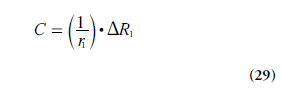
where r₁ is the longitudinal CA relaxivity. It is normally assumed that r₁ is independent of the compartment in which the CA resides, but one should be aware that this might not always be entirely correct [84,85]. Although the relationship between MRI signal and CA concentration is nonlinear and often rather complex, the CA concentration can be derived if the relationship between the CA-induced T₁ change and the corresponding alteration of the MRI signal S is established and explicit. A reasonably ambitious DCE-MRI experiment would require estimation of CA concentration in a supplying artery (i.e., the AIF) as well as in the tissue of interest, and it may be challenging to accurately estimate such a large range of CA concentrations. In quantitative DCE-MRI, a two-step approach for data acquisition is often employed (Figure 7), including an initial quantification of T₁ before CA administration (often referred to as baseline T₁), and the dynamic scan (e.g., using the SPGR), which includes acquisition of a few pre-CA images (giving the baseline signal) and a series of images during and up to several minutes after the CA injection. Acquisition of a B₁-map is frequently included in the DCE-MRI imaging protocol.

T₁ is estimated from the baseline and dynamic measurements, using appropriate signal equations, and the concentration of CA is obtained using Equation 29. Regarding the baseline T₁ quantification, T₁ measurements can broadly be categorized as either inversion/saturation recovery prepared sequences or variable saturation techniques. In DCE-MRI, it is common to estimate T₁ by variable flip angle gradient-echo image acquisitions, normally with constant TR [86]. This approach is relatively fast and offers good tissue coverage in multislice or 3D volume mode [87].

Estimation of uncertainties in DCE-MRI estimates is far from straightforward. The measured signal intensity over time depends on the specific pulse sequence and the setting of relevant imaging parameters (TE, TR, flip angle and so on), according to a given signal equation, and the signal data are noisy and sampled with limited temporal resolution. Furthermore, the baseline T₁ estimate also suffers from errors related to the specific T₁-measurement approach [88]. All these factors are likely to introduce bias and/or uncertainty in the CA concentration estimates. Thereafter, a pharmacokinetic model is fitted to the suboptimal concentration estimates, and a variety of physiological parameters, for example, Ktrans, TBF, ve and vp are extracted with various precision and accuracy. Measurement errors propagate in a highly nontrivial way during the different steps of mathematical processing, and the resulting error is also likely to depend on the absolute value, over a physiologically relevant range, of the parameter of interest. A typical example of DCE-MRI data is given in Figure 8.

It is not feasible to provide general estimates of accuracy and precision, but a number of investigations have been published regarding the uncertainty and reliability of various DCEMRI protocols and kinetic models [89–93]. For the SPGR sequence, Schabel and Parker [92] concluded that optimization of, in particular, flip angle and baseline signal accuracy enabled significantly improved effective signal-to-noise ratio and decreased sensitivity to errors in flip angle and baseline T₁ when estimating the CA concentration. However, in the T₁ quantification, it is still important to consider, for example, B₁ inhomogeneity [94], imperfect SPGR radiofrequency spoiling [95] and slice profile imperfections [87]. Inclusion of corrections for imperfect radio-frequency spoiling in the SPGR signal equation may be beneficial [96].

Currently, one of the most important and challenging issues in quantitative DCE-MRI is the measurement of the AIF. Several early implementations of DCE-MRI and modeling of CA kinetics tended to refrain from using individually measured AIFs, but instead employed the experimentally simpler solution of a population- averaged AIF [75]. However, it was soon recognized that individual AIF measurements are warranted [97], because the exact AIF shape depends on CA injection rate and dose, cardiac output, CA distribution pattern in the body and renal function. It is clear that AIF errors propagate to result in inaccurate pharmacological parameters [98], and an AIF measurement specific to a given subject and examination is generally superior [99]. Examples of challenges in the AIF measurement, in addition to the general quantification problems mentioned above, are sufficient temporal resolution (of the order of 1–1.5 s), accurate quantification of peak concentrations [100], arterial partial volume effects [101], inflow effects [83] and arterial dispersion between the site of measurement and the tissue region of interest [53]. One potential solution is to employ a separate injection of a small amount of CA, prior to the actual dynamic study and to measure the AIF during this pre-bolus experiment [102–104]. This approach enables tailoring of the imaging protocol to the AIFmeasurement requirements and it also includes the advantage of lowering the peak concentration, which reduces the risk of signal saturation or nonlinearity. Another alternative is to employ dual-contrast sequences, for example, interleaved acquisition of an inversion-prepared T₁-weighted image and a T₁/T₂^*-mixed-weighted image for determination of the AIF [105]. Finally, phasebased AIFs (Figure 8) and venous output functions show considerable promise due to excellent phase shift-versus-concentration linearity and favorable signal-to-noise ratio [47,106] but might not be entirely trivial to acquire in realistic patient materials, particularly not over the extended time periods required in DCE-MRI [104].

Another topic that has received considerable attention in DCE-MRI is the potential effect of water exchange between tissue compartments. CA quantification in DCE-MRI normally assumes the conditions of the fast-exchange limit, in other words, molecular motion between spaces being rapid (and/or relaxation time difference between spaces being small), which leads to an observed effect of relaxation that approaches a single average value. For normal, relatively low, concentrations of CA in the interstitial space, the assumption of fast exchange between the intracellular and interstitial spaces was supported by experiments by Donahue et al. [107], but exchange conditions have indeed been under some debate [108], and exchange effects are dependent on the employed imaging parameters of the pulse sequence [109]. Intravascular-to-interstitial (i.e., transendothelial) water exchange is more likely to depart from the fast-exchange limit, since the difference in longitudinal relaxation rate between the intra- and extra-vascular compartment may be prominent, for example, initially after CA administration or if the CA remains intravascular (such as in the brain) [110]. With large first-pass extraction, the effect of slow exchange is likely to be limited, but it should at least be considered in brain applications [101].

Finally, imaging strategies for T1-weighted first-pass imaging, applied to, for example, cardiovascular and cerebral perfusion MRI, should be briefly mentioned. Various imaging strategies exist for myocardial perfusion imaging, but SPGR (although being somewhat slow), hybrid EPI (with echo train lengths of 3–6 echoes) as well as magnetization preparation by saturation recovery followed by a steadystate free precession pulse sequence for readout are well-known examples [111,112]. The modelfree deconvolution approach mentioned above (Equation 4) has been applied, for example, to myocardial blood flow [113] as well as CBF [114,115] assessment. In the brain applications, Larsson et al. used a saturation recovery gradient recalled sequence both for baseline T1 measurements and for subsequent dynamic imaging [114,115].

CT

Assessment of perfusion and permeability by DCE-CT using the Tofts, extended Tofts or AATH models is quite feasible (e.g., see [116]). In this context, an obvious advantage of using DCE-CT is the absence of any water exchangerelated problems, which cannot be ruled out in DCE-MRI, and a comparative tracer-kinetic analysis of corresponding data from both DCEMRI and DCE-CT, has in fact been proposed for assessment of the magnitude of water exchange effects in DCE-MRI [117]. There is also an increasing and well-founded interest in CT-based myocardial perfusion imaging [118].

Future perspective

In DSC-MRI, quantification of CBV and CBF in absolute terms is a challenging task, particularly due to the complicated issue of varying T₂^* relaxivities in blood and tissue, and a subjectspecific calibration by a separate CBV or CBF estimate (either global or from selected regions), obtained by an independent perfusion technique, might be a viable way to proceed. Recent advances in quantification of magnetic susceptibility using MRI phase information might turn out to be beneficial also for CA concentration quantification in vivo [119]. For DSC-MRI as well as dynamic perfusion CT, a possible extension of the data analysis is to extract additional information from the tissue residue curve or the corresponding transit-time distribution in connection with assessment of cerebral oxygen extraction and metabolism [120].

Perfusion and permeability studies by DCEMRI and DCE-CT are likely to become of considerable value in connection with evaluation of early treatment response in a number of cancer therapy modalities [4]. Furthermore, tailored or individualized therapy is a current keyword in oncology, and identification of particularly aggressive parts of an individual tumor by functional medical imaging would be of great benefit. In this context, one should emphasize the need for standardization and consensus with regard to imaging protocols and model parameter extraction. The focus of the current overview has primarily been on standard tracerkinetic models, applied to MRI, but it is clear that so-called second-generation models, for example, returning separate estimates of TBF and capillary permeability, are likely to become increasingly important in dynamic MRI and CT applications [121].

In cardiac imaging, perfusion CT techniques are likely to represent an important future advancement [118]. Cardiac CT shows good availability and it already provides excellent anatomical and angiographic information. The possibility of adding myocardial perfusion studies, at rest and during stress, would certainly be beneficial. Stress myocardial perfusion CT shows promising results, although further validation and optimization of the technique is required [122].

Acknowledgements

A Bibic, M Bolognese, A Garpebring, R Kern and R Siemund are gratefully acknowledged for providing valuable illustrations.

Financial & competing interests disclosure

This work was supported by the Swedish Research Council (grant no. 13514). The author has no other relevant affiliations or financial involvement with any organization or entity with a financial interest in or financial conflict with the subject matter or materials discussed in the manuscript apart from those disclosed.

No writing assistance was utilized in the production of this manuscript.

References

Papers of special note have been highlighted as:
* of interest
** of considerable interest

1. Wintermark M, Sesay M, Barbier E et al. Comparative overview of brain perfusion imaging techniques. Stroke 36, 83–99 (2005).
2. Jackson A, Buckley DL, Parker GJ (Eds). Dynamic Contrast-Enhanced Magnetic Resonance Imaging in Oncology. Springer, Berlin, Germany (2005). & Important textbook covering most dynamic MRI techniques and illustrating how they are applied in different organs.
3. Awasthi R, Rathore RK, Soni P et al. Discriminant analysis to classify glioma grading using dynamic contrast-enhanced MRI and immunohistochemical markers. Neuroradiology 54(3), 205–213 (2012).
4. Zahra M, Hollingsworth K, Sala E, Lomas D, Tan L. Dynamic contrast-enhanced MRI as a predictor of tumour response to radiotherapy. Lancet Oncol. 8, 63–74 (2007).
5. Lassen NA, Perl W. Tracer Kinetic Methods in Medical Physiology. Raven Press, NY, USA (1979). & Classic and excellent textbook with all relevant definitions.
6. Fung YC. Biodynamics: Circulation. Springer-Verlag, NY, USA (1984).
7. Klabunde RE. Cardiovascular Physiology Concepts (2nd Edition). Lippincott Williams & Wilkins, PA, USA (2012).
8. Meier P, Zierler KL. On the theory of the indicator-dilution method for measurement of blood flow and volume. J. Appl. Physiol. 6, 731–744 (1954).
9. Fick A. Über die messung des blutquantums in der herzventrikel. Verhandl. Phys. Med. Ges. Wurzburg 2, XVI (1870).
10. Zierler KL. Equations for measuring blood flow by external monitoring of radioisotopes. Circ. Res. 16, 309–321 (1965).
11. Brix G, Salehi Ravesh M, Zwick S, Griebel J, Delorme S. On impulse response functions computed from dynamic contrast-enhanced image data by algebraic deconvolution and compartmental modeling. Phys. Med. 28(2), 119–128 (2012).
12. Meier P, Zierler KL. On the theory of the indicator-dilution method for measurement of blood flow and volume. J. Appl. Physiol. 6, 731–744 (1954).
13. Rempp KA, Brix G, Wenz F, Becker CR, Gückel F, Lorenz WJ. Quantification of regional cerebral blood flow and volume with dynamic susceptibility contrast-enhanced MR imaging. Radiology 193, 637–641 (1994). & Early article providing a straightforward recipe on how to perform deconvolutionbased cerebral blood flow quantification by dynamic susceptibility contrast (DSC)-MRI.
14. Cenic A, Nabavi DG, Craen RA, Gelb AW, Lee TY. Dynamic CT measurement of cerebral blood flow: a validation study. Am. J. Neuroradiol. 20(1), 63–73 (1999).
15. Zierler KL. Theoretical basis of indicatordilution methods for measuring flow and volume. Circ. Res. 10, 393–407 (1962).
16. Wirestam R, Andersson L, Østergaard L et al. Assessment of regional cerebral blood flow by dynamic susceptibility contrast MRI using different deconvolution techniques. Magn. Reson. Med. 43(5), 691–700 (2000).
17. Larson KB, Perman WH, Perlmutter JS, Gado MH, Ollinger JM, Zierler K. Tracer-kinetic analysis for measuring regional cerebral blood flow by dynamic nuclear magnetic resonance imaging. J. Theor. Biol. 170(1), 1–14 (1994).
18. Gobbel GT, Fike JR. A deconvolution method for evaluating indicator-dilution curves. Phys. Med. Biol. 39(11), 1833–1854 (1994).
19. Østergaard L, Weisskoff RM, Chesler DA, Gyldensted C, Rosen BR. High resolution measurement of cerebral blood flow using intravascular tracer bolus passages. Part I: Mathematical approach and statistical analysis. Magn. Reson. Med. 36(5), 715–725 (1996). & Consitutes the breakthrough for DSC-MRI, in particular owing to its introduction of a robust singular value decomposition approach for deconvolution.
20. Andersen IK, Szymkowiak A, Rasmussen CE et al. Perfusion quantification using Gaussian process deconvolution. Magn. Reson. Med. 48(2), 351–361 (2002).
21. Zanderigo F, Bertoldo A, Pillonetto G, Cobelli C. Nonlinear stochastic regularization to characterize tissue residue function in bolus-tracking MRI: assessment and comparison with SVD, block-circulant SVD, and Tikhonov. IEEE Trans. Biomed. Eng. 56(5), 1287–1297 (2009).
22. Wu O, Østergaard L, Weisskoff RM, Benner T, Rosen BR, Sorensen AG. Tracer arrival timing-insensitive technique for estimating flow in MR perfusion-weighted imaging using singular value decomposition with a block-circulant deconvolution matrix. Magn. Reson. Med. 50(1), 164–174 (2003). & Important supplement to [19] since this paper introduced a delay-insensitive singular value decomposition deconvolution algorithm.
23. Rosen BR, Belliveau JW, Vevea JM, Brady TJ. Perfusion imaging with NMR contrast agents. Magn. Reson. Med. 14, 249–265 (1990).
24. Benner T, Reimer P, Erb G et al. Cerebral MR perfusion imaging: first clinical application of a 1 M gadolinium chelate (Gadovist 1.0) in a double-blinded randomized dose-finding study. J. Magn. Reson. Imaging 12(3), 371–380 (2000).
25. Tombach B, Benner T, Reimer P et al. Do highly concentrated gadolinium chelates improve MR brain perfusion imaging? Intraindividually controlled randomized crossover concentration comparison study of 0.5 versus 1.0 mol/l gadobutrol. Radiology 226(3), 880–888 (2003).
26. Thilmann O, Larsson EM, Björkman- Burtscher IM, Ståhlberg F, Wirestam R. Comparison of contrast agents with high molarity and with weak protein binding in cerebral perfusion imaging at 3 T. J. Magn. Reson. Imaging 22(5), 597–604 (2005).
27. Alger JR, Schaewe TJ, Lai TC et al. Contrast agent dose effects in cerebral dynamic susceptibility contrast magnetic resonance perfusion imaging. J. Magn. Reson. Imaging 29, 52–64 (2009).
28. Griffiths PD, Pandya H, Wilkinson ID, Hoggard N. Sequential dynamic gadolinium magnetic resonance perfusion-weighted imaging: effects on transit time and cerebral blood volume measurements. Acta Radiol. 47(10), 1079–1084 (2006).
29. Gauden AJ, Phal PM, Drummond KJ. MRI safety: nephrogenic systemic fibrosis and other risks. J. Clin. Neurosci. 17, 1097–1104 (2010).
30. Villringer A, Rosen BR, Belliveau JW et al. Dynamic imaging with lanthanide chelates in normal brain: contrast due to magnetic susceptibility effects. Magn. Reson. Med. 6(2), 164–174 (1988).
31. Boxerman JL, Hamberg LM, Rosen BR, Weisskoff RM. MR contrast due to intravascular magnetic susceptibility perturbations. Magn. Reson. Med. 34(4), 555–566 (1995).
32. Simonsen CZ, Østergaard L, Smith DF, Vestergaard-Poulsen P, Gyldensted C. Comparison of gradient- and spin-echo imaging: CBF, CBV, and MTT measurements by bolus tracking. J. Magn. Reson. Imaging 12(3), 411–416 (2000).
33. Speck O, Chang L, DeSilva NM, Ernst T. Perfusion MRI of the human brain with dynamic susceptibility contrast: gradient-echo versus spin-echo techniques. J. Magn. Reson. Imaging 12(3), 381–387 (2000).
34. Heiland S, Kreibich W, Reith W et al. Comparison of echo-planar sequences for perfusion-weighted MRI: which is best? Neuroradiology 40, 216–221 (1998).
35. 35 Kjølby BF, Østergaard L, Kiselev VG. Theoretical model of intravascular paramagnetic tracers effect on tissue relaxation. Magn. Reson. Med. 56(1), 187–197 (2006). & Very important study for understanding the complex T2* relaxivity issue in DSC-MRI, with in vivo transverse relaxivities being different between tissue and artery.
36. 36 Newman GC, Hospod FE, Patlak CS et al. Experimental estimates of the constants relating signal change to contrast concentration for cerebral blood volume by T2* MRI. J. Cereb. Blood Flow Metab. 26(6), 760–770 (2006).
37. 37 Schmiedeskamp H, Straka M, Newbould RD et al. Combined spin- and gradient echo perfusion-weighted imaging. Magn. Reson. Med. 68(1), 30–40 (2012).
38. 38 Pedersen M, Klarhöfer M, Christensen S. Quantitative cerebral perfusion using the PRESTO acquisition scheme. J. Magn. Reson. Imaging 20(6), 930–940 (2004).
39. 39 Calamante F, Vonken EJ, van Osch MJ. Contrast agent concentration measurements affecting quantification of bolus-tracking perfusion MRI. Magn. Reson. Med. 58(3), 544–553 (2007).
40. 40 Kiselev VG. On the theoretical basis of perfusion measurements by dynamic susceptibility contrast MRI. Magn. Reson. Med. 46(6), 1113–1122 (2001).
41. 41 Engvall C, Ryding E, Wirestam R et al. Human cerebral blood volume (CBV) measured by dynamic susceptibility contrast MRI and 99mTc-RBC SPECT. J. Neurosurg. Anesthesiol. 20(1), 41–44 (2008).
42. 42 Grandin CB, Bol A, Smith AM, Michel C, Cosnard G. Absolute CBF and CBV measurements by MRI bolus tracking before and after acetazolamide challenge: repeatability and comparison with PET in humans. Neuroimage 26(2), 525–535 (2005).
43. 43 Knutsson L, Börjesson S, Larsson EM et al. Absolute quantification of cerebral blood flow in normal volunteers: correlation between Xe-133-SPECT and dynamic susceptibility contrast MRI. J. Magn. Reson. Imaging 26(4), 913–920 (2007).
44. 44 van Osch MJ, Vonken EP, Viergever MA, van der Grond J, Bakker CJ. Measuring the arterial input function with gradient echo sequences. Magn. Reson. Med. 49, 1067–1076 (2003).
45. 45 Calamante F, Connelly A, van Osch MJ. Nonlinear ΔR2* effects in perfusion quantification using bolus-tracking MRI. Magn. Reson. Med. 61, 486–492 (2009).
46. 46 Bleeker EJ, van Buchem MA, van Osch MJ. Optimal location for arterial input function measurements near the middle cerebral artery in first-pass perfusion MRI. J. Cereb. Blood Flow Metab. 29(4), 840–852 (2009).
47. 47 Akbudak E, Conturo TE. Arterial input functions from MR phase imaging. Magn. Reson. Med. 36, 809–815 (1996).
48. 48 Ellinger R, Kremser C, Schocke MFH et al. The impact of peak saturation of the arterial input function on quantitative evaluation of dynamic susceptibility contrast-enhanced MR studies. J. Comput. Assist. Tomogr. 24(6), 942–948 (2000).
49. 49 Vonken EP, van Osch MJ, Bakker CJ, Viergever MA. Measurement of cerebral perfusion with dual-echo multi-slice quantitative dynamic susceptibility contrast MRI. J. Magn. Reson. Imaging 10(2), 109–117 (1999).
50. 50 Rausch M, Scheffler K, Rudin M, Radu EW. Analysis of input functions from different arterial branches with γ variate functions and cluster analysis for quantitative blood volume measurements. Magn. Reson. Imaging 18(10), 1235–1243 (2000).
51. 51 Chen JJ, Smith MR, Frayne R. The impact of partial-volume effects in dynamic susceptibility contrast magnetic resonance perfusion imaging. J. Magn. Reson. Imaging 22(3), 390–399 (2005).
52. 52 van Osch MJ, Vonken EP, Bakker CJ, Viergever MA. Correcting partial volume artifacts of the arterial input function in quantitative cerebral perfusion MRI. Magn. Reson. Med. 45(3), 477–485 (2001).
53. 53 Calamante F, Gadian DG, Connelly A. Delay and dispersion effects in dynamic susceptibility contrast MRI: simulations using singular value decomposition. Magn. Reson. Med. 44, 466–473 (2000). & A study highlighting the inherent problem of arterial dispersion when using intravascular tracers.
54. 54 Willats L, Christensen S, Ma HK, Donnan GA, Connelly A, Calamante F. Validating a local arterial input function method for improved perfusion quantification in stroke. J. Cereb. Blood Flow Metab. 31(11), 2189–2198 (2011).
55. 55 Willats L, Connelly A, Calamante F. Improved deconvolution of perfusion MRI data in the presence of bolus delay and dispersion. Magn. Reson. Med. 56(1), 146–156 (2006).
56. 56 Boxerman JL, Schmainda KM, Weisskoff RM. Relative cerebral blood volume maps corrected for contrast agent extravasation significantly correlate with glioma tumor grade, whereas uncorrected maps do not. AJNR Am. J. Neuroradiol. 27(4), 859–867 (2006).
57. 57 Aronen HJ, Gazit IE, Louis DN et al. Cerebral blood volume maps of gliomas: comparison with tumor grade and histologic findings. Radiology 191, 41–51 (1994).
58. 58 Gall P, Mader I, Kiselev VG. Extraction of the first bolus passage in dynamic susceptibility contrast perfusion measurements. Magn. Reson. Mater. Phys. 22(4), 241–249 (2009).
59. 59 Østergaard L, Johannsen P, Høst-Poulsen P et al. Cerebral blood flow measurements by magnetic resonance imaging bolus tracking:comparison with [15O]H2O positron emission tomography in humans. J. Cereb. Blood Flow Metab. 18, 935–940 (1998).
60. 60 Shin W, Cashen TA, Horowitz SW, Sawlani R, Carroll TJ. Quantitative CBV measurement from static T1 changes in tissue and correction for intravascular water exchange. Magn. Reson. Med. 56(1), 138–145 (2006).
61. 61 Axel L. Cerebral blood flow determination by rapid-sequence computed tomography: a theoretical analysis. Radiology 137(3), 679–686 (1980). & A very early introduction to cerebral blood flow measurement by diagnostic imaging equipment.
62. 62 Wintermark M, Maeder P, Thiran JP, Schnyder P, Meuli R. Quantitative assessment of regional cerebral blood flows by perfusion CT studies at low injection rates: a critical review of the underlying theoretical models. Eur. Radiol. 11(7), 1220–1230 (2001).
63. 63 Cianfoni A, Colosimo C, Basile M, Wintermark M, Bonomo L. Brain perfusion CT: principles, technique and clinical applications. Radiol. Med. 112, 1225–1243 (2007).
64. 64 Singh J, Daftary A. Iodinated contrast media and their adverse reactions. J. Nucl. Med. Technol. 36, 69–74 (2008).
65. 65 Quaia E. Assessment of tissue perfusion by contrast-enhanced ultrasound. Eur. Radiol. 21, 604–615 (2011).
66. 66 Kern R, Perren F, Schoeneberger K, Gass A, Hennerici M, Meairs S. Ultrasound microbubble destruction imaging in acute middle cerebral artery stroke. Stroke 35, 1665–1670 (2004).
67. 67 Powers J, Averkiou M, Bruce M. Principles of cerebral ultrasound contrast imaging. Cerebrovasc. Dis. 27(Suppl. 2), S14–S24 (2009).
68. 68 Dijkmans PA, Visser CA, Kamp O. Adverse reactions to ultrasound contrast agents: is the risk worth the benefit? Eur. J. Echocardiogr. 6(5), 363–366 (2005).
69. 69 Gauthier M, Tabarout F, Leguerney I et al. Assessment of quantitative perfusion parameters by dynamic contrast-enhanced sonography using a deconvolution method: an in vitro and in vivo study. J. Ultrasound Med. 31(4), 595–608 (2012).
70. 70 Kern R, Diels A, Pettenpohl J et al. Real-time ultrasound brain perfusion imaging with analysis of microbubble replenishment in acute MCA stroke. J. Cereb. Blood Flow Metab. 31(18), 1716–1724 (2011).
71. 71 Sourbron SP, Buckley DL. On the scope and interpretation of the Tofts models for DCE-MRI. Magn. Reson. Med. 66(3), 735–745 (2011).
72. 72 Crone C. The permeability of capillaries in various organs as determined by use of the indicator diffusion method. Acta Physiol. Scand. 58, 292–305 (1963).
73. 73 Renkin EM. Exchangeability of tissue potassium in skeletal muscle. Am. J. Physiol. 197, 1211–1215 (1959).
74. 74 Larsson HB, Stubgaard M, Frederiksen JL, Jensen M, Henriksen O, Paulson OB. Quantitation of blood–brain barrier defect by magnetic resonance imaging and gadolinium-DTPA in patients with multiple sclerosis and brain tumors. Magn. Reson. Med. 16(1), 117–131 (1990).
75. 75 Tofts PS, Kermode AG. Measurement of the blood–brain barrier permeability and leakage space using dynamic MR imaging. 1. Fundamental concepts. Magn. Reson. Med. 17, 357–367 (1991).
76. 76 Brix G, Semmler W, Port R, Schad LR, Layer G, Lorenz WJ. Pharmacokinetic parameters in CNS Gd-DTPA enhanced MR imaging. J. Comput. Assist. Tomogr. 15(4), 621–628 (1991).
77. 77 Tofts PS, Brix G, Buckley DL et al. Estimating kinetic parameters from dynamic contrast-enhanced T1-weighted MRI of a diffusable tracer: standardized quantities and symbols. J. Magn. Reson. Imaging 10(3), 223–232 (1999). & Very important and clarifying paper on dynamic contrast-enhanced MRI, which summarized a number of early studies and standardized the relevant terminology.
78. 78 Kety SS. The theory and applications of the exchange of inert gas at the lungs and tissues. Pharmacol. Rev. 3(1), 1–41 (1951).
79. 79 Tofts PS. Modeling tracer kinetics in dynamic Gd-DTPA MR imaging. J. Magn. Reson. Imaging 7, 91–101 (1997).
80. 80 Johnson JA, Wilson TA. A model for capillary exchange. Am. J. Physiol. 210, 1299–1303 (1966).
81. 81 St Lawrence KS, Lee TY. An adiabatic approximation to the tissue homogeneity model for water exchange in the brain: I. Theoretical derivation. J. Cereb. Blood Flow Metab. 18(12), 1365–1377 (1998).
82. 82 Kershaw LE, Cheng HL. Temporal resolution and SNR requirements for accurate DCE-MRI data analysis using the AATH model. Magn. Reson. Med. 64(6), 1772–1780 (2010).
83. 83 Garpebring A, Wirestam R, Östlund N, Karlsson M. Effects of inflow and radiofrequency spoiling on the arterial input function in dynamic contrast-enhanced MRI: a combined phantom and simulation study. Magn. Reson. Med. 65(6), 1670–1679 (2011).
84. 84 Stanisz, GJ, Henkelman RM. Gd-DTPA relaxivity depends on macromolecular content. Magn. Reson. Med. 44, 665–667 (2000).
85. 85 Haar PJ, Broaddus WC, Chen ZJ, Fatouros PP, Gillies GT, Corwin FD. Gd-DTPA T1 relaxivity in brain tissue obtained by convection-enhanced delivery, magnetic resonance imaging and emission spectroscopy. Phys. Med. Biol. 55(12), 3451–3465 (2010).
86. 86 Cheng HM, Wright GA. Rapid highresolution T1 mapping by variable flip angles: accurate and precise measurements in the presence of radiofrequency field inhomogeneity. Magn. Reson. Med. 55(3), 566–574 (2006).
87. 87 Brookes JA, Redpath TW, Gilbert FJ, Murray AD, Staff RT. Accuracy of T1 measurement in dynamic contrast-enhanced breast MRI using two- and three-dimensional variable flip angle fast low-angle shot. J. Magn. Reson. Imaging 9(2), 163–171 (1999).
88. 88 Deoni SC. Quantitative relaxometry of the brain. Top. Magn. Reson. Imaging 21, 101–113 (2010).
89. 89 Buckley DL. Uncertainty in the analysis of tracer kinetics using dynamic contrastenhanced T1-weighted MRI. Magn. Reson. Med. 47, 601–606 (2002).
90. 90 Dale BM, Jesberger JA, Lewin JS, Hillenbrand CM, Duerk JL. Determining and optimizing the precision of quantitative measurements of perfusion from dynamic contrast enhanced MRI. J. Magn. Reson. Imaging 18, 575–584 (2003).
91. 91 Kershaw LE, Buckley DL. Precision in measurements of perfusion and microvascular permeability with T1-weighted dynamic contrast-enhanced MRI. Magn. Reson. Med. 56(5), 986–992 (2006).
92. 92 Schabel MC, Parker DL. Uncertainty and bias in contrast concentration measurements using spoiled gradient echo pulse sequences. Phys. Med. Biol. 53(9), 2345–2373 (2008).
93. 93 De Naeyer D, De Deene Y, Ceelen WP, Segers P, Verdonck P. Precision analysis of kinetic modelling estimates in dynamic contrast enhanced MRI. Magn. Reson. Mater. Phys. 24(2), 51–66 (2011).
94. 94 Treier R, Steingoetter A, Fried M, Schwizer W, Boesiger P. Optimized and combined T1 and B1 mapping technique for fast and accurate T1 quantification in contrastenhanced abdominal MRI. Magn. Reson. Med. 57(3), 568–576 (2007).
95. 95 Preibisch C, Deichmann R. Influence of RF spoiling on the stability and accuracy of T1 mapping based on spoiled FLASH with varying flip angles. Magn. Reson. Med. 61(1), 125–135 (2009).
96. 96 Yarnykh VL. Optimal radiofrequency and gradient spoiling for improved accuracy of T1 and B1 measurements using fast steady-state techniques. Magn. Reson. Med. 63(6), 1610–1626 (2010).
97. 97 Evelhoch JL. Key factors in the acquisition of contrast kinetic data for oncology. J. Magn. Reson. Imaging 10(3), 254–259 (1999).
98. 98 Cheng HL. Investigation and optimization of parameter accuracy in dynamic contrastenhanced MRI. J. Magn. Reson. Imaging 28(3), 736–743 (2008).
99. 99 Ashton E, Raunig D, Ng C, Kelcz F, McShane T, Evelhoch J. Scan-rescan variability in perfusion assessment of tumors in MRI using both model and data-derived arterial input functions. J. Magn. Reson. Imaging 28(3), 791–796 (2008).
100. 100 Sourbron S, Michaely HJ, Reiser MF, Schoenberg SO. MRI-measurement of perfusion and glomerular filtration in the human kidney with a separable compartment model. Invest. Radiol. 43(1), 40–48 (2008).
101. 101 Sourbron S, Ingrisch M, Siefert A, Reiser M, Herrman K. Quantification of cerebral blood flow, cerebral blood volume, and blood– brain-barrier leakage with DCE-MRI. Magn. Reson. Med. 62, 205–217 (2009).
102. 102 Köstler H, Ritter C, Lipp M, Beer M, Hahn D, Sandstede J. Prebolus quantitative MR heart perfusion imaging. Magn. Reson. Med. 52, 296–299 (2004).
103. 103 Kershaw LE, Cheng HLM. A general dual-bolus approach for quantitative DCE-MRI. Magn. Reson. Imaging 29(2), 160–166 (2011).
104. 104 Garpebring A, Wirestam R, Yu J, Asklund T, Karlsson M. Phase-based arterial input functions in humans applied to dynamic contrast-enhanced MRI: potential usefulness and limitations. Magn. Reson. Mater. Phys. 24(4), 233–245 (2011).
105. 105 Prochnow D, Beyersdorff D, Warmuth C, Taupitz M, Gemeinhardt O, Lüdemann L. Implementation of a rapid inversion-prepared dual-contrast gradient echo sequence for quantitative dynamic contrast-enhanced magnetic resonance imaging of the human prostate. Magn. Reson. Imaging 23(10), 983–990 (2005).
106. 106 Foottit C, Cron GO, Hogan MJ, Nguyen TB, Cameron I. Determination of the venous output function from MR signal phase: feasibility for quantitative DCE-MRI in human brain. Magn. Reson. Med. 63(3), 772–781 (2010).
107. 107 Donahue KM, Burstein D, Manning WJ, Gray ML. Studies of Gd-DTPA relaxivity and proton exchange rates in tissue. Magn. Reson. Med. 32(1), 66–76 (1994).
108. 108 Yankeelov TE, Rooney WD, Li X, Springer CS Jr. Variation of the relaxographic ‘shutter-speed’ for transcytolemmal water exchange affects the CR bolus-tracking curve shape. Magn. Reson. Med. 50(6), 1151–1169 (2003).
109. 109 Donahue KM, Weisskoff RM, Chesler DA. Improving MR quantification of regional blood volume with intravascular T1 contrast agents: accuracy, precision, and water exchange. Magn. Reson. Med. 36(6), 858–867 (1996).
110. 110 Larsson HB, Rosenbaum S, Fritz-Hansen T. Quantification of the effect of water exchange in dynamic contrast MRI perfusion measurements in the brain and heart. Magn. Reson. Med. 46(2), 272–281 (2001).
111. 111 Schwitter J. Myocardial perfusion. J. Magn. Reson. Imaging 24, 953–963 (2006).
112. 112 Jerosch-Herold M. Quantification of myocardial perfusion by cardiovascular magnetic resonance. J. Cardiovasc. Magn. Reson. 12, 57 (2010).
113. 113 Jerosch-Herold M, Swingen C, Seethamraju RT. Myocardial blood flow quantification with MRI by model-independent deconvolution. Med. Phys. 29, 886–897 (2002).
114. 114 Larsson HBW, Hansen AE, Berg HK, Rostrup E, Haraldseth O. Dynamic contrast-enhanced quantitative perfusion measurement of the brain using T1-weighted MRI at 3T. J. Magn. Reson. Imaging 27, 754–762 (2008).
115. 115 Larsson HB, Courivaud F, Rostrup E, Hansen AE. Measurement of brain perfusion, blood volume, and blood–brain barrier permeability, using dynamic contrast-enhanced T1-weighted MRI at 3 Tesla. Magn. Reson. Med. 62(5), 1270–1281 (2009).
116. 116 Korporaal JG, van Vulpen M, van den Berg CA, van der Heide UA. Tracer kinetic model selection for dynamic contrast-enhanced computed tomography imaging of prostate cancer. Invest. Radiol. 47(1), 41–48 (2012).
117. 117 Bains LJ, McGrath DM, Naish JH et al. Tracer kinetic analysis of dynamic contrastenhanced MRI and CT bladder cancer data: a preliminary comparison to assess the magnitude of water exchange effects. Magn. Reson. Med. 64(2), 595–603 (2010).
118. 118 Marcus RP, Nikolaou K, Theisen D, Reiser MF, Bamberg F. Myocardial perfusion imaging by computed tomography: today and tomorrow. Int. J. Clin. Pract. Suppl. 65, 14–22 (2011).
119. 119 Wharton S, Bowtell R. Whole-brain susceptibility mapping at high field: a comparison of multiple- and singleorientation methods. Neuroimage 53(2), 515–525 (2010).
120. 120 Jespersen SN, Østergaard L. The roles of cerebral blood flow, capillary transit time heterogeneity, and oxygen tension in brain oxygenation and metabolism. J. Cereb. Blood Flow Metab. 32(2), 264–277 (2012).
121. 121 Sourbron SP, Buckley DL. Tracer kinetic modelling in MRI: estimating perfusion and capillary permeability. Phys. Med. Biol. 57(2), R1–R33 (2012). 122 Techasith T, Cury RC. Stress myocardial CT perfusion: an update and future perspective. JACC Cardiovasc. Imaging 4(8), 905–916 (2011).