Research Article - Imaging in Medicine (2019) Volume 11, Issue 6
Advanced neural network solution for detection of lung pathology and foreign body on chest plain radiographs
Lilian Nitris1, Evgenii Zhukov2, Dmitry Blinov2*, Pavel Gavrilov3, Ekaterina Blinova4,5 and Alina Lobishcheva61Research and Development Department, 910 Foulk Road, Suite 201, Wilmington, DE 19803, USA
2Department of Medical Sciences, 10, 2nd Tverskoy-Yamskoy Lane, Moscow, 125047 Russia
3Department of Radiology, Saint-Petersburg Research Institute of Phthisiopulmonology, 2-4 Ligovsky Prospekt, St. Petersburg, 191040, Russia
4Department of Operative Surgery and Clinical Anatomy, Sechenov University, 8/2 Trubetzkaya Street, Moscow, 119991 Russia
5Faculty Surgery Department, National Research Mordovia State University, 68, Bolshevistskaya Street, Saransk, 430005 Russia
6Department of Oncology and Radiology, Saint-Petersburg State University, 7-9 Universitetskaya Embankment, St. Petersburg, 199034 Russia
- Corresponding Author:
- Dmitry Blinov
Department of Medical Sciences
10 2nd Tverskoy-Yamskoy Lane
Moscow 125047 Russia
E-mail: d.blinov@cmai.team
Abstract
Objective : An approach was suggested to detect whether patient has any lung pathology or not.
Materials and Methods : The approach was based on neural networks-aided analysis of chest X-ray frontal images. The neural network ensemble included 15 neural networks. Some of them were trained to analyze different parts of chest area, e.i. heart, diaphragm, lungs and related parts. And the other set of networks were trained to describe another meta-data of X-rays, such as patient position (laying or standing), quality of image, etc. The set of outputs of every model was aggregated with boosting model then. Result of model prediction was presented as probability of lung pathology on radiograph. Another 2 models were described in this article as parts of suggested approach. One of these model was trained to detect if there any foreign body within chest area on X-ray image or not. Another one was trained to classify which kind of foreign body was visualized (after first model gave positive prediction). To train models 9093 frontal X-ray images were used. Those images were labeled by group of radiologist.
Results : The study showed that both foreign bodies detection and classification models demonstrated satisfactory results. The weak part of both models was precision for negative classes (those classes are “non-medical artefact” for one model and “foreign body is not visualized” for the other one). But it was not so critical for such kind of tasks.
Conclusions : the model may be used to help a practitioner make decision whether a patient needs additional diagnostics or not.
Keywords
neural network ■ artificial intelligence ■ lung pathology ■ foreign body ■ detection
Introduction
Chest X-ray is the most common radiological diagnostic method in the world, which accounts for up to 45% of all radiologic studies [1]. The wide availability of the method is due to its low cost and great diagnostic potential in relation to such socially significant pathologies as tuberculosis, lung cancer and pneumonia [2]. At the same time, radiography is an example of diagnostic ambiguity. The reason for this is that a planar image is formed as a result of the imposition of anatomical structures having different structure, composition and density. As a result, the image may contain dozens of signs encountered in hundreds of pathological processes and conditions [2]. This leads to difficulties in reading and interpretation of the X-ray picture, the occurrence of discrepancies between the diagnosticians, and ultimately leads to often unreasonable additional clarifying examinations.
Medical errors are currently considered along with cardiovascular and oncological diseases as the leading cause of mortality in the world [3]. According to a number of authors, in the USA, deaths due to medical errors account for 44 thousand to 400 thousand cases per year [4,5]. Additional costs from budgets of all levels associated with medical errors, according to WHO estimates, fluctuate between 17 and 29 billion US dollars annually. The frequency of false-negative results in the analysis of chest radiographs in developed countries is on average 4% [6,7], while the probability of error in identifying individual radiological phenomena does not fall below 30% since 1949, when Garland published his first observational study [8]. According to a retrospective observation del Ciello et al. (2017), devoted to the problem of X-ray diagnosis of lung cancer, the frequency of detection of identifiable focal lesions in the lungs up to 30 mm in size does not exceed 29% and increases to 82% only with an increase in the size of the lesion to 40 mm [9].
Recent years have been marked by breakthrough solutions in the field of machine processing of medical data, including diagnostic images. In particular, the use of neural networks, parabolic, vector regression models was proposed for the diagnosis of lung diseases [10]. Chronic bronchial obstructive conditions and pneumonia were suggested to be diagnosed using a combination of a neural network solution and an artificial immune system [11]; Algorithms have been developed for the diagnosis of tuberculosis, lung cancer and pneumonia based on segmentation using the decision tree, the Bayesian principle [12]. The mentioned approaches were successfully used to classify pathological conditions, however, their accuracy, specificity and sensitivity, as well as their productivity, were inferior to the methods of deep machine learning that came to replace them [13,14]. Neural networks (competitive, back propagation errors, convolutional) have demonstrated advantages over humans in the accuracy of interpretation and its speed. The subsequent use of neural network capabilities to solve the problems of detecting individual pathological conditions in medical images allowed us to create high-performance models [15,16]. The purpose of this work is to develop neural network-based solution to detect whether patient has any lung pathology or not.
Materials and Methods
■ Ethics
The study protocol was reviewed and approved independently by Bio-ethic Commission of Saint-Petersburg Research Institute of Phthisiopulmonology on March 23, 2019 (Report No. 19/10-534) and Ethic Committee of Saint-Petersburg State University on February 17, 2019 (Review No. 15561). An informed consent for using chest X-ray image has been received from all patients, study participants, whose images composed digital archives of the Clinics.
■ Source of radiographs
We used 276840 frontal X-ray images of lungs. One part of them, 112120 frontal labeled radiographs from the hospitals affiliated to National Institutes of Health Clinical Center (USA), was obtained from free open access database [17]. The other images were extracted from digital archives of St. Petersburg State University Clinical Hospital (SPSUCH), Clinics of St. Petersburg Research Institute of Phthysiopulmonology (CSPRIP) and Sechenov University Pulmonology Clinic (SUPC). The images distribution is shown at TABLE 1.
| Source of images | Size of dataset, images | Number of labeled images |
|---|---|---|
| SPSUCH | 77439 | 77439 |
| CSPRIP | 53514 | 5689 |
| SUPC | 33767 | 10096 |
Table 1. Sources of not-open access chest X-ray images, used in the study.
■ X-ray labeling procedure
All collected images were randomly assigned at 7:3 ratios to training and testing sets respectively. Radiographs used for the CNN training were labeled by 5 equally-educated and well-experienced radiologists with more than 10 years at a position (each image by single practitioner). The images were blindly designated to the radiologist’s personal account in Care Mentor labeling software particularly developed for the study and secured by login and password. Labeling process comprised consequently logging in, browsing through the images pending list, viewing an image and choosing specific attributes that characterize condition of lungs and presence of foreign bodies, according to a protocol. Special medical documentation (protocol) was designed to label data. This protocol has as fields with multiple choice as filed with single choice from few cases. Every field of protocol was used to get labeled data to train every separate neural network. The software allowed the radiologists correct their options until the data having sent to the image preprocessing.
At testing stage of the study each X-ray image was labeled independently by two radiologists chosen blindly. It made possible further consideration of the CNN and the radiologist’s results divergence as well as variability of the practitioners’ opinion [18].
■Proposed workflow
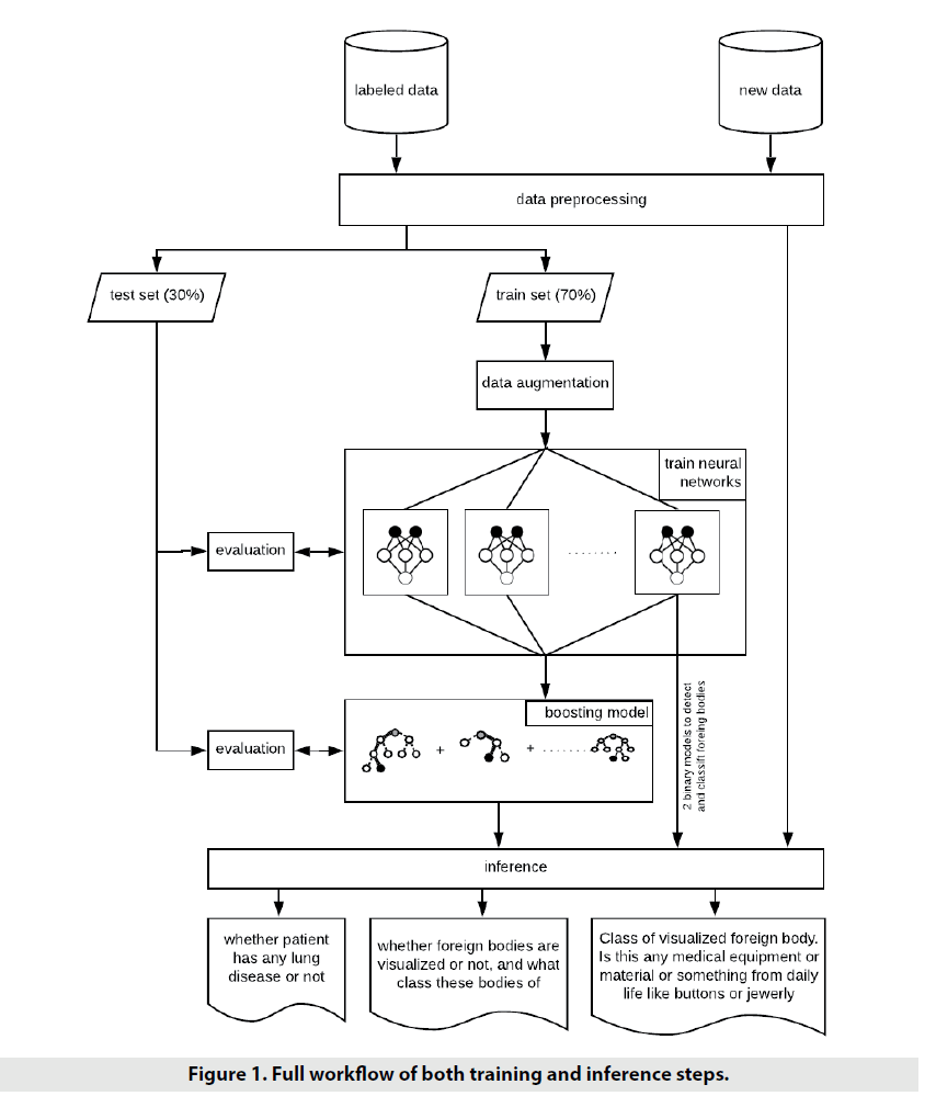
Approached workflow is shown on FIGURE 1 Basically the first step of various machine learning and deep learning workflows is data preprocessing. Preprocessing can be specific from training neural network to evaluate it. For example, image resizing is used for both training and evaluating steps, but training step also can require additional work on data - so called image augmentation [19] (the set of various random image modifications) to diversify source dataset and, as a result, make model to be more robust and efficient in prediction.
After data was preprocessed and split up into train and test subsets, it was time to training step. At the beginning, the stack of neural networks was to be trained. And then trained neural networks were used to train boosting model.
Finally, inference step was implemented. Predictions from neural networks and boosting model were obtained.
■Data pre-processing
Every single model was trained regardless to another models. Thus, preprocessing workflow was a little bit different from model to model. For example, some subsets of models required special image size than another (TABLE 2). All used size settings were: 224 × 224; 299 × 299 or 512 × 512. Also different normalization algorithms were applied within different models. Some models required inputs values being in range [-1,1], but another in [0,1]. There are two ways to normalize pixel values to be appropriate as neural networks inputs (1):
| No | Neural network | Pre-processing | Architecture |
|---|---|---|---|
| 1 | Simple binary classification: - patient doesn’t have any lung pathology; - patient probably have some lung pathology. |
Resize: 224 x 224 Normalizing: inpt = img / 255.0 |
- base model: InceptionV3 before bottleneck and with Global Average Pooling in the end; - Dense layer (1024 units and ReLU as activation); - Dense layer (1 unit and sigmoid as activation). |
| 2 | Binary classification. Patient position: - standing; - lying. |
Resize: 224 x 224 Normalizing: inpt = img / 255.0 |
- base model: ResNet-50 before bottleneck and without pooling; - Flatten layer (all features after convolutional layers are used without pooling); - Dense layer (512 units and ReLU as activation); - Dense layer (1 unit and sigmoid as activation). |
| 3 | Binary classification. X-ray image quality: - satisfactory; - not satisfactory. |
Resize: 512 x 512 Normalizing: inpt = img / 127.5 - 1 |
- base model: InceptionV3 before bottleneck and with Global Average Pooling in the end; - Dropout with rate = 0.5 - Dense layer (2 units and softmax as activation). |
| 4 | Binary classification. Are any foreign bodies visualized: - no; - yes. |
Resize: 512 x 512 Normalizing: inpt = img / 127.5 - 1 |
- base model: InceptionV3 before bottleneck and with Global Average Pooling in the end; - Dropout with rate = 0.5 - Dense layer (2 units and softmax as activation). |
| 5 | Binary classification. Is there any pathology of pleural cavity: - no; - yes. |
Resize: 512 x 512 Normalizing: inpt = img / 127.5 - 1 |
- base model: InceptionV3 before bottleneck and with Global Average Pooling in the end; - Dropout with rate = 0.5 - Dense layer (2 units and softmax as activation). |
| 6 | Binary classification. Is there any pathology of lung fields: - no; - yes. |
Resize: 512 x 512 Normalizing: inpt = img / 127.5 - 1 |
- base model: InceptionV3 before bottleneck and with Global Average Pooling in the end; - Dropout with rate = 0.5 - Dense layer (2 units and softmax as activation). |
| 7 | Multiclass classification of possible aorta pathology: - pathology not found; - unwrapped; - extended; - sclerotic; - dense. |
Resize: 512 x 512 Normalizing: inpt = img / 127.5 - 1 |
- base model: InceptionV3 before bottleneck and with Global Average Pooling in the end; - Dropout with rate = 0.5 - Dense layer (5 units and softmax as activation). |
| 8 | Multiclass classification of possible diafragma changes: - pathology not found; - edges are not clear; - changed. |
Resize: 512 x 512 Normalizing: inpt = img / 127.5 - 1 |
- base model: InceptionV3 before bottleneck and with Global Average Pooling in the end; - Dropout with rate = 0.5 - Dense layer (3 units and softmax as activation). |
| 9 | Multiclass classification of possible heart pathology: - pathology not found; - edges are unclear; - extended across; - extended to the left. |
Resize: 512 x 512 Normalizing: inpt = img / 127.5 - 1 |
- base model: InceptionV3 before bottleneck and with Global Average Pooling in the end; - Dropout with rate = 0.5 - Dense layer (4 units and softmax as activation). |
| 10 | Multiclass classification of possible lung roots pathology: - pathology not found; - unclear; - unstructured; - extended. |
Resize: 512 x 512 Normalizing: inpt = img / 127.5 - 1 |
- base model: InceptionV3 before bottleneck and with Global Average Pooling in the end; - Dropout with rate = 0.5 - Dense layer (4 units and softmax as activation). |
| 11 | Binary classification. Are there pleural adhesions: - no; - yes. |
Resize: 512 x 512 Normalizing: inpt = img / 127.5 - 1 |
- base model: InceptionV3 before bottleneck and with Global Average Pooling in the end; - Dropout with rate = 0.5 - Dense layer (2 units and softmax as activation). |
| 12 | Binary classification. Are there any changes of lung pattern: - no; - yes. |
Resize: 512 x 512 Normalizing: inpt = img / 127.5 - 1 |
- base model: InceptionV3 before bottleneck and with Global Average Pooling in the end; - Dropout with rate = 0.5 - Dense layer (2 units and softmax as activation). |
| 13 | Binary classification. Does patient have pneumonia: - no; - yes. |
Resize: 512 x 512 Normalizing: inpt = img / 127.5 - 1 |
- base model: InceptionV3 before bottleneck and with Global Average Pooling in the end; - Dropout with rate = 0.5 - Dense layer (2 units and softmax as activation). |
| 14 | Multiclass classification of possible lung lung disease: - pathology not found; - pneumosclerosis; - pneumothorax; - emphysema; - pneumofibrosis; - hydrothorax. |
Resize: 512 x 512 Normalizing: inpt = img / 127.5 - 1 |
- base model: InceptionV3 before bottleneck and with Global Average Pooling in the end; - Dropout with rate = 0.5 - Dense layer (6 units and softmax as activation). |
| 15 | Binary classification. Is any focus visualized: - no; - yes. |
Resize: 512 x 512 Normalizing: inpt = img / 255.0 |
- base model: InceptionV3 before bottleneck and without pooling; - Flatten layer (all features after convolutional layers are used without pooling); - Dropout with rate = 0.4 - Dense layer (1024 units and ReLU as activation); - Dropout with rate = 0.4 - Dense layer (512 units and ReLU as activation); - Dropout with rate = 0.3 - Dense layer (1 unit and sigmoid as activation). |
| 16 | Binary classification. Does visualized body belong to medical equipment / materials : - no; - yes. |
Resize: 512 x 512 Normalizing: input = img / 127.5 - 1 |
- base model: InceptionV3 before bottleneck and with Global Average Pooling in the end; - Dropout with rate = 0.5 - Dense layer (2 units and softmax as activation). |
Table 2. Stack of models used as input for boosting.
input = source_image / 127.5 - 1
(for range [-1, 1]);
input = source_image / 255.0
(for range [0, 1]) (1)
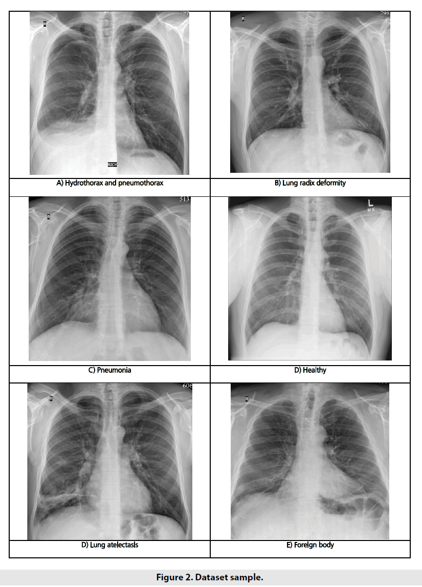
Our input images had significantly various resolution, different contrast and brightness levels, detailing quality and noise rates. Some images given in prepared grayscale compressed format (*.png or *.jpg), but some of them were present in raw DICOM format and required to be converted to be fit for sending to neural network. Examples of the input images are shown in FIGURE 2.
Resizing step was different for some models. But there were some common steps to apply on data before fit models with them. Few data augmentation steps [19], such as translation, rotation, sharpening, weak affine transformations, contrast and brightness changes and addition of Gaussian noise were applied to increase the diversity of the training data. After all dataset was splitted into subsets to train models and evaluate them relatively by 70% and 30%. Images of test sample were not used for the network training process.
■ Model architecture
Suggested solution was not just one model, but stack of models followed by one boosting model to aggregate outputs of all models of this stack. The full stack of models with architecture features are described in TABLE 2. Every model consists of pretrained part and additional classification part (some set of layers). Pre-trained part is model, which has already been trained on big dataset like ImageNet [20]. Usually, such models are used as backbone for custom neural network. Top classification layer or layers were replaced by custom ones. Approached solution uses such models as Inception-V3 [21] and ResNet-50 [22] as base pretrained models. Every record in TABLE 2 describes particular purpose of every neural network, base (or backbone) model architecture it uses and custom layers applied after convolutional (features extraction) part of base model.
Predicted outputs of all stacked neural networks – probabilities vectors – are concatenated in new feature vector then. Boosting model uses this new feature vector as input to predict only one value – whether patient has any lung pathology or not. XGBoost model was used as boosting model [18].
■ Training process
We took two steps to train our models. The first one included the stack of neural network models training processes, while on the other one we trained the boosting model. Input images and their corresponding label maps were used to train every neural network. Every model requires own set of labels. All neural networks were trained with Adam optimizer with β1=0.9 and β2=0.999. The initial learning rate was chosen to be 0.001 and were reduced by 10 times if loss function stopped to improve during 10 epochs. Also early stopping was applied to stop training process if loss function was not improved during 15 epochs.
Binary cross entropy (2) were used as loss function in cases of sigmoid function as neural network output. If softmax was used as output of neural network, then categorical cross entropy (3) was as followed:
Loss binary_crossentropy=-(ylog(p(y)+(1-y) log(1-p(y))),
y – was true label for instance (positive or negative); p(y) – predicted label (value from range [0; 1]), probability of positive label.
Loss categorical_crossentropy=-c=1Cyclog(p(yc))
yc = 1, if c was class for instance, 0 – otherwise; p(yc) – predicted value, probability for instance to belong to c-class
XGBoost model was used as boosting model. Input of boosting model: 39-dimensional vector composed from neural networks stack outputs. Output – confidence rate that patient had any lung pathology. Model parameters were optimized with cross-validation. As a training result, model got max_depth=7 and eta=0.1. Another parameter of model is set by its default values. More information about XGBoost model and its parameters had been documented before [18].
■Post-processing
Raw output of HPC was value from range [0,1], where ‘0–pathology is not found’, ‘1– probably patient has any lung pathology’. To make final decision it is required to set threshold value. In terms of this work threshold was set to find right balance between ROC AUC, recall score for pathology class and precision score for healthy class. After experiments threshold was set to 0.4 to achieve satisfied balance. This means that patient has lung pathology if output of aggregation model is equal or higher than 0.4, otherwise patient is thought to be healthy.
Quality measurement
To evaluate the models, we used few metrics: AUC (Area Under the Curve) ROC (Receiver Operating Characteristics), recall and precision. In binary classification, precision (4) (also called positive predictive value) is the fraction of relevant instances among the retrieved instances, while recall (5) (also known as sensitivity) is the fraction of relevant instances that have been retrieved over the total amount of relevant instances:
Recall = TPTP+FN (4)
Precision = TPTP+FP (5)
where: TP – number of instances classified as positive class correctly, FP – number of instances classified as positive class incorrectly, and FN – number of instances classified as negative class incorrectly.
If model was evaluated related to pathology class, then pathology class was considered to be positive class. And healthy was positive class when model was evaluated related to healthy class.
During evaluation and parameter optimization more attention was paid for recall score, for pathology score and precision score for healthy class, both to reduce false-healthy cases.
AUC (Area Under the Curve) ROC (Receiver Operating Characteristics) curve is another metric which can be very important to evaluate binary classification model. Basically it tells how much model is capable of distinguishing between classes. By other words - higher the AUC ROC, better the model is at predicting healthy as healthy and pathology as pathology. Calculating AUC ROC consists of 2 stages:
• Calculating values of True Positive Rate (TPR) and False Positive Rate (FPR) with different decision threshold (from 0 to 1) - coordinates for curve - ROC part.
• Calculating the area of figure formed by ROC curve and both X and Y axis (TPR and FPR) - AUC part. The higher AUC ROC - the better quality model has. Also analysis of ROC curve can help to achieve desired balance between TPR and FPR by varying threshold.
Results
After models had been trained the following quality metrics values were achieved (TABLE 3). Section “Results” describes qualities metrics calculated in relation to default decision threshold = 0.5 for foreign bodies models and 0.4 for Normal-Pathology binary classification model. For Normal-Pathology binary classification model it meant that we considered patient to have any lung pathology if model outcome was equal or higher 0.4.
| Model | |||
|---|---|---|---|
| metric | Normal-Pathology Binary Classification Model positive: normal negative: pathology |
Foreign Bodies Binary Classification Model positive: foreign bodies are visualized negative: foreign bodies are not visualized |
Kind of Foreign Body. Binary Classification Model positive: visualized body belongs to any medical material or equipment negative: visualized body doesn’t belong to any medical material or equipment |
| recall (for positive) | 0.7912 | 0.9489 | 0.9278 |
| recall (for negative) | 0.7411 | 0.9374 | 0.9231 |
| precision (for positive) | 0.6777 | 0.969 | 0.9570 |
| precision (for negative) | 0.8376 | 0.8989 | 0.8898 |
| AUC ROC | 0.7662 | 0.9432 | 0.9377 |
Table 3. Quality metrics for suggested trained models.
As we said above, value of threshold equaling 0.4 was chosen to get satisfied a balance between recall for positive class and precision for negative class. Such balance decreases number of patients wrongly considered as healthy patients, and at the same time increase of total number of recognized patients who probably has any lung pathology. As a result, as less patients were labeled to normal class, as more patient were labeled to pathology class. Despite the fact that it can lead to overdiagnostics, such approach is required to avoid miss-labeling patients with pathology to normal class.
Another 2 models also were used out of stack to detect whether any foreign body was visualized on X-ray image to classify it. We can notice that both foreign bodies detection and classification models show satisfactory results. The weak part of both models is precision for negative classes (those classes are “non-medical body” for one model and “foreign body is not visualized” for another one). But it’s not so critical for such kind of tasks.
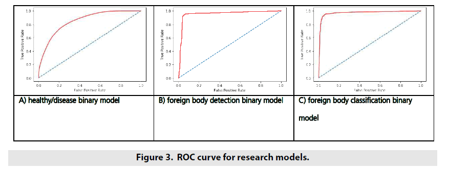
ROC curve is another way to demonstrate model’s ability to distinguish different classes in binary classification tasks. ROC curves for developed models are shown in FIGURE 3.
Discussion and Conclusion
During research, set of models were developed to analyze chest radiographs. Whole set of models was stacked to build one binary classification model to detect whether patient had any lung disease or not. Talking about quality analysis with ROC curve, we could observe quite high quality of Foreign Bodies models judged by big area under ROC curve – top-left corner of the curve was close to be right. Pathology-Normal model did not possess such high quality. Smooth curve (as a result, smaller area under the curve) told us about it.
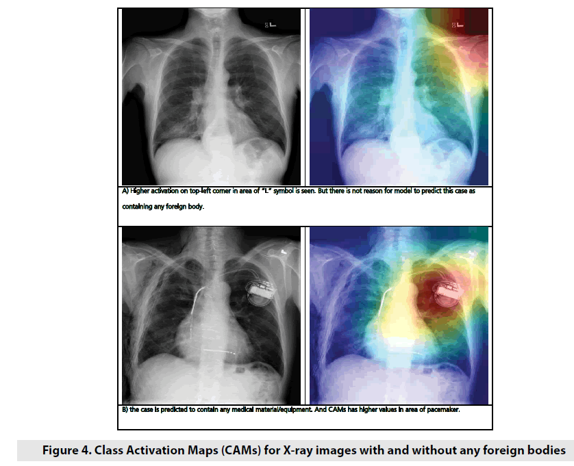
As an example to demonstrate how the neural network activates for X-ray images with and without foreign bodies, Class Activation Maps (CAM) for 2 random images were applied (FIGURE 4). CAMs are used to demonstrate which neurons of layer were more active for particular image and particular class. Sometimes it helps to understand which part of image neural network pay more attention on during making decision process. As it’s observed on picture above, neural network showed higher activation values on places which are not normal for normal state of lungs. To classify foreign body, we used 2-steps approach: at the 1st step we detect if any foreign body is visualized on X-ray image, and at the 2nd step we classify foreign body if one or more were detected.
As further work it’s possible to research another approaches. For example, we can try 2 separate models: one of them can detect whether any medical material or equipment is detected on image, and another model can be trained to detect if any non-medical foreign body is detected.
The model may be used to help a practitioner make decision whether a patient needs additional diagnostics or not.
References
- Yao L, Poblenz E, Dagunts D et al. Learning to diagnose from scratch by exploiting dependencies among labels. Comput. Soc. Conf. Comput. Vis. Pattern. Recognit. 1: 1-18, (2018).
- Sabih DE, Sabih A, Sabih Q et al. Image perception and interpretation of abnormalities; can we believe our eyes? Can we do something about it? Insights. Imaging. 2: 47-55, (2011).
- Makary MA, Daniel M. Medical error: the third leading cause of death in the US. BMJ. 353: 2139, (2016).
- Kohn LT, Corrigan JM, Donaldson MS et al. To err is human: building a safer health system. Washington, DC: National. Academies. Press. 287: 1- 312, (2000).
- Busby LP, Courtier JL, Glastonbury CM. Bias in radiology: the How and Why of misses and misinterpretation. Radiographics. 38: 236-247, (2018).
- Waite S, Scott J, Gale J et al. Interpretative error in radiology. AJR. 208: 739-749, (2017).
- Ropp A, Waite S, Reede D et al. Did I miss that: subtle and commonly missed findings on chest radiographs. Curr. Probl. Diagn. Radiol. 44: 277-289, (2015).
- Garland LH. On the scientific evaluation of diagnostic procedures. Radiol. 52: 309-328, (1949).
- Del Ciello A, Franchi D, Contegiacomo A et al. Missed lung cancer: when, where, and why? Diagn. Interv. Radiol. 23: 118-126, (2017).
- Er O, Yumusak N, Temurtas F. Chest diseases diagnosis using artificial neural networks. Expert. Sys. Appl. 37: 7648-7655, (2010).
- Er O, Sertkaya C, Temurtas F et al. A comparative study on chronic obstructive pulmonary and pneumonia diseases diagnosis using neural networks and artificial immune system. J. Med. Sys. 33: 485-492, (2009).
- Khobragade S, Tiwari A, Pati CY et al. Automatic detection of major lung diseases u sing chest radiographs and classification by feed-forward artificial neural network. Proceedings of 1st IEEE International Conference on Power Electronics. Intelligent. Control. Energy. Systems. 16: 1-5, (2016).
- Litjens G, Kooi T, Bejnordi EB et al. A survey on deep learning in medical image analysis. Med. Image. Analysis. 42: 60-88, (2017).
- Albarqouni S, Baur C, Achilles F et al. Aggnet: deep learning from crowds for mitosis detection in breast cancer histology images. IEEE. Transact. Med. Imag. 35: 1313-1321, (2016).
- Avendi MR, Kheradvar A, Jafarkhani H. A combined deep-learning and deformable-model approach to fully automatic segmentation of the left ventricle in cardiac MRI. Med. Image. Analysis. 30: 108-119, (2016).
- Shin HC, Roberts K, Lu L et al. Learning to read chest X-rays: recurrent neural cascade model for automated image annotation. IEEE. Comput. Soc. Conf. Comput. Vis. Pattern. Recognit, 16: 2497-2506, (2016).
- Wang XS, Peng YF, Lu L et al. ChestX-ray8: hospital-scale chest x-ray database and benchmarks on weakly-supervised classification and localization of common thorax diseases. IEEE. Conf. Comput. Vis. Pattern. Recognit. 14: 3462-3471, (2017).
- https://xgboost.readthedocs.io/en/latest/index.html
- Shorten C, Khoshgoftaar A. Survey on Image Data Augmentation for Deep Learning. TMJ. Big. Data. 6: 60, (2019).
- Deng J, Dong W, Socher R et al. ImageNet: A Large-Scale Hierarchical Image Database. IEEE Comput. Vis. Pattern. Recognit (2009.l
- Szegedy C, Vanhoucke V, Ioffe S et al. Rethinking the Inception Architecture for Computer Vision. IEEE Comput. Vis. Pattern. Recognit 2016; 308.
- He K, Zhang X, Ren S et al. Deep residual learning for image recognition. IEEE Comput. Soc. Conf. Comput. Vis. Pattern. Recognit. 16: 770-778, (2016).
