Review Article - Interventional Cardiology (2021) Volume 13, Issue 1
Relaxation along fictitious field with rank n (RAFFn): A promising magnetic resonance imaging method to determine myocardial infarction
- Corresponding Author:
- Timo Liimatainen
Research Unit of Medical Imaging, Physics and Technology,
University of Oulu,
P.O.Box 5000,
FI-90014,
Oulu,
Finland
E-mail: timo.liimatainen@oulu.fi
Received date: October 30, 2020 Accepted date: November 23, 2020 Published date: November 30, 2020
Abstract
Purpose of this review: Cardiovascular Diseases (CVD) are the leading cause of deaths worldwide. Myocardial Infarction (MI) is one of the deadliest CVDs. MI is causing many complex cellular biological changes in the myocardium after myocardial infarction (MI). Modern magnetic resonance imaging (MRI) techniques, such as rotating frame relaxation time T1ρ, can be used to visualize and quantify the damages in the myocardium after the MI and for the detection of myocardial alternations without the use of contrast agents. However, T1ρ method suffers from high specific absorption rate i.e. tissue heating. Modern MRI technique called Relaxation Along a Fictitious Field (RAFF) in the Rotating Frame of Rank n (RAFFn) has overcome the specific absorption rate problems of T1ρ method. Additionally, RAFFn has been shown to visualize and quantify the MI in both preclinical and clinical studies.
Recent findings: The RAFFn method has been used to characterize the MI in preclinical mouse MI models with promising results. The RAFFn method was implemented in standard clinical 1.5 T magnet for characterizing MI in human patients. The RAFFn has been used to determine also the fibrosis in preclinical hypertrophic cardiomyopathy mouse model and the results revealed the sensitiveness of RAFFn method to hypertrophic cardiomyopathy-related tissue changes in the myocardium.
Summary: RAFFn has been used to characterize myocardial infarction in humans and in mice. RAFFn owns potential to be used in the MI diagnosis without contrast agents.
Keywords
RAFFn; T1ρ; MRI; Myocardial infarction
Introduction
Non-invasive medical imaging has a vital role in the diagnosis and follow-up of cardiovascular diseases (CVDs), which are the leading cause of death in the Western countries [1]. One disease with high mortality in CVD is myocardial infarction (MI), which is caused by a blockage of the coronary artery [1]. The blockage of the coronary artery due to thrombosis leads to the absence of perfusion causing the loss of myocytes, inflammation, granulation tissue formation, fibrosis and remodeling of the damaged tissues [1]. This unwanted biological chain can cause arrhythmia and eventually sudden death [1]. In this review, we describe how modern imaging techniques in Magnetic Resonance Imaging (MRI) can be used to characterize the MI and following myocardial remodeling.
Cardiac anatomy and its function can be imaged with ultrasound, computed tomography (CT) and MRI [2,3]. The advantages of MRI over ultrasound is the capability to image the anatomy, the function and the myocardium properties, whereas ultrasound is able to image only the anatomy and the function of the heart [2,3]. Additionally, the advantages of MRI over current conventional radiation- and nuclear-based cardiac imaging techniques include a high soft tissue contrast and lack of exposure to ionizing radiation [2]. MRI has become an important non-invasive tool to accurately characterize properties of myocardium in vivo such as conventional longitudinal relaxation (T1) and transversal relaxation (T2) relaxation time mapping. Other endogenous contrasts, such as methods utilizing relaxation in rotating frame including longitudinal relaxation in the rotating frame (T1ρ) and Relaxation Along a Fictitious Field in the rank n (RAFFn), are providing more detailed information about slow molecular motions and fluctuations in the different pathological states and changes [2]. Therefore, MRI can be used beneficially with high flexibility in several ways for imaging of biological tissues and it is a safe imaging modality to characterize the modifications of the heart.
For the recap, magnetization (M) is formed by the sum of individual spin angular momentums, which are precessing with near Larmor frequency ω0=γB0, where γ is the gyromagnetic ratio, around the external static magnetic field (B0) and the direction of M is along the laboratory z axis [4,5]. When the M is formed, spin angular momentums are in thermal equilibrium [4,5]. This thermal equilibrium needs to be perturbed with an external burst of energy to allow the detection of the signal [4,5]. This burst of energy is done with radiofrequency (RF) electromagnetic pulse [4,5]. After the external energy burst, spin angular momentums are relaxing back to the thermal equilibrium and this phenomenom is called relaxation [4,5].
Relaxation in the rotating frame of reference was introduced by Redfield in the NMR field in 1955 [6,7] and later in the MRI field in 1985 by Sepponen et al. [8]. The term rotating frame of reference arises from the fact that it rotates around the laboratory z axis with the Larmor frequency. Meanwhile, the M is visualized to be stationary in rotating frame of reference similarly as RF field (B1) given on-resonance. Here rotating frame of reference is denoted as x’, y’ and z’. Longitudinal relaxation time constant in the rotating frame is called T1ρ [8] and similarly transversal relaxation time constant in the rotating frame is T2ρ [9]. The simplest form of T1ρ measurement is the on-resonance spin-lock (SL) measurement, where M is the first flipped to the xy-plane and M is then locked with the RF pulse for a specific time duration, which is called the time-spin-lock (TSL). T1ρ relaxation time can be measured either using continuous wave [10], continuous wave rotary echo [11], adiabatic techniques [12] or gradient modulated adiabatic pulses [13]. However, one critical limitation of all techniques of T1ρ is its relatively high specific absorption rate (SAR) [14], which describes the energy absorbed into tissue i.e. heating of the tissue during the imaging [14].
One option to reduce SAR in the rotating frame relaxation measurements is RAFF [15]. RAFF is an advanced rotating frame relaxation time measurement where the relaxation of M occurs along, a final effective field, which consists of B1, off-resonance and a fictitious magnetic field [16]. The original existence of a fictitious field phenomena was detected in low frequency NMR experiments in 1957 [17] and it took over 40 years when frequency sweep in designing of adiabatic pulses came into NMR [18] and extra 10 years to that to introduce the fictitious field phenomena into highfield MRI relaxation time measurements in 2010 [15].
Physics of RAFF Method
In rotating frame (x’,y’,z’), B1 (ω1=γB1) is applied on-resonance (the
Larmor frequency) appears along the x’ [4,5]. In case of adiabatic
pulses, the rotating frame is often defined so that the rotation
follows RF pulse off-resonance from the Larmor frequency [15].
In that case, the B1 is able to stay on x’ axis although RF pulse
off-resonance is varying. Then a time-dependent field component
`ΔB0(t) arises into direction of z’ axis from difference between
Larmor and RF pulse frequencies ![]()
When RF pulse is applied with off-resonance, M nutates around a sum field (H1) consisting of B1 and ΔB0(t) components with amplitude (Equation 1).

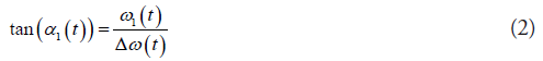
Depending on B1 and ΔB0(t), the H1 orientation angle related to z’ axis is (Equation 2)
If M is placed initially along H1 and H2 orientation varies so that adiabatic condition (dα1/dt << H1) is fulfilled, M follows H1 orientation (Figure 1A).

Figure 1: The coordinate system of 1A: 1st (x’, y’, z’) and 2nd (x’’, y’’, z’’) rotating frames and 1B: 2nd and partly 3rd (x’’’, y’’’, z’’’) rotating frames. Notice that z’’ is parallel with H1 and z’’’ is along with H2.
If this condition is intentionally violated, and the frequency sweep of H1 changes fast, M is not able to follow H1. A fast sweep of H1 into x’z’ plane generates a fictitious magnetic field component dα1/ dt (≡ C1) along the Y axis.
H1 and dα1/dt together form a final effective field (H2), which is a geometrical sum of H1 (≡ D1) and (≡ C1) (Figure 1B) and therefore, the amplitude of H2 is a vector sum of its components (Equation 3).

Now, M is placed initially along H2, which keeps the M locked along final effective field H2. When using sine amplitude modulation and cosine frequency modulation as RF pulse wave form, a time invariant dα1/dt amplitude can be created, which is a base of RAFF2 method [15].
To help to understand the concept of RAFF2 method, it is useful to move from the first to the second rotating frame (x’’, y’’, z’’), which nutates around y’ (=y’’) (Figure 2) with angular velocity of dα1/dt. The angle between H2 and z’’ is (Equation 4)

Figure 2: A schematic view from the rotating frames of rank n=1 to 4 used to describe RAFFn.

The pulse duration (Tp) for RAFF2 method is selected so that during the pulse, M rotates from laboratory z axis to xy plane (90° pulse) [19]. Therefore, Tp for RAFF2 method is defined as (Equation 5)
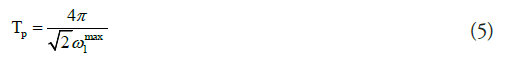
In the original publication, the power of RAFF2 pulse was defined as  leading to Tp of 2.26 ms [15].
RAFF2 pulse consists of four segments of RF amplitude and frequency modulations, which are marked as P (Figure 3). The first P rotates M 90° to xy plane. The second segment, a time inversion pulse P-1, with π phase shift compared to P brings the M back to the z’’ axis [19,20]. To further compensate imperfections arising from B0 inhomogeneity PP-1 is repeated with π phase shift leading to a PP-1 PπPπ-1 refocusing scheme with the total length of TP [19,20]. An important detail in the RAFF2 method is that the fictitious field increases the final effective field amplitude without increasing the RF power and SAR.

Figure 3: A schematic view of the RAFF2 pulse sequence with an Adiabatic Full-Passage (AFP) inversion pulse in front of RAFF2 sequence. RAFF2 can be measured also without the AFP inversion pulse. The inset describes the amplitude and phase modulations of RAFF2 pulse.
The M can be determined for both initial conditions along z axis (M+0) or along -z axis (M-0) in the RAFF2 measurement with the following (Equation 6)
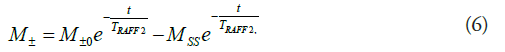
where MSS is the steady-state of M, TRAFF2 is RAFF2 relaxation time and t is time. Steady-state M is formed in RAFF2 due to a periodical pattern of RF pulse and therefore, MSS needs to be taken into account in the fitting of the relaxation time [15].
RAFF2 method can be expanded by making H2 field time dependent [15,21]. The next transformation will be performed around x’’ axis and the next transformation after that around the y’’’ axis (Figure 2). The amplitude of the final effective field for RAFFn can be calculated by (Equation 7)

and the angle between Hn and zn is given by (Equation 8)
When n increases, the fraction of B1 component decreases if the amplitude of the final effective field is kept constant. The decreased B1 is important since SAR is related to B1. Another feature of increasing n is the tolerance for frequency off-set due to refocusing the M [22], and therefore the increase of the tolerance for both B0 and B1 inhomogeneities is increased. The SAR values with the same effective field ranges are significantly lower in the RAFFn method compared to the T1ρ measurement, which is an advantage of the RAFFn over T1ρ [19]. Lower SAR values become more obvious with the higher ranks [19].
Results
RAFFn in mouse myocardial infarction and hypertrophy models in vivo at high (9.4 T) magnetic field
Our group has used the RAFFn method to determine the MI area in a few studies. Since the RAFFn is rotating frame relaxation method similarly as T1ρ, TRAFFn relaxation time is sensitive to slow molecular motions, which occur in the frequency range of 0.1 to 5 kHz. It has been demonstrated that TRAFFn mapping can determine accurately the MI area from its surroundings (Figure 4A) [23]. The RAFF2 and RAFF4 were applied to characterize the MI area in various time points after the MI and TRAFF2 relaxation time was found to increased significantly up to 7 days and remain elevated until day 21 after the MI in infarct area (Figure 4B). Also, TRAFF4 relaxation time was significantly elevated at all-time points compared to the remote area in the infarct area [23]. To study accuracy of infarct size determined with RAFFn, an area of overestimation (AOE) of infarct area, which based on the difference between area with increased TRAFF2 relaxation time and area with increased signal in late gadolinium enhancement (LGE) was calculated [23]. The AOE value of TRAFF2 was the lowest of all relaxation times measured in the study (TRAFF2, TRAFF4, T1ρ and T2) indicating that area of increased TRAFF2 was the closest to the LGE [23]. Additionally, correlations were drawn between MI sizes based increased relaxation times or LGE signal intensities and infarct areas based on Sirius red stained histology-images. The MI areas from TRAFF2 (R2=0.93, P<0.001) and TRAFF4 (R2 =0.94, P<0.001) exhibited the highest correlations as well as LGE (R2=0.92, P<0.01) [23].

Figure 4: Relaxation times measured in study [23] are shown 1A: Visually at the last time point and 1B: As a function of time. Statistical analyses were done with two-way ANOVA with Bonferroni’s post-hoc test (*P<0.05, **P<0.01, ***P<0.001) to test the significance between day-1 and other time points and also between the MI and remote areas.
The TRAFF2 and TRAFF4 were measured also in insufficient lymphatic system MI mouse model one week after the MI [24]. TRAFF2 and TRAFF4 significantly differentiated the composition of MI area in insufficient lymphatic myocardium compared to normal myocardium with effective lymphatic system whereas; these changes in MI areas were not detected with conventional T2 or T1ρ relaxation times [24].
TRAFFn mapping has been used to determine the fibrosis in hypertrophic myocardium mouse model, where the hypertrophic myocardium was induced by increasing heart workload by transverse aortic constriction (TAC) and mice were imaged in several time points after the operation [25]. The TRAFF2 and TRAFF3 were found to be more sensitive than T1ρ mapping detect hypertrophic cardiomyopathy-related tissue changes in the myocardium [25]. The myocardial fibrosis was verified by Masson’s trichrome histology staining [25].
RAFFn in Human MI at 1.5 T Magnetic Field
RAFFn method have been implemented in standard clinical 1.5 T magnet for characterizing MI in human patients [26]. The study revealed that RAFF2 and RAFF3 methods with steady state (SS) included in the data analysis is feasible in humans with MI (Figure 5). Fairly high Spearman correlation (R2=0.64, P<0.01) between MI size based on TRAFF3, SSRAFF3 and extracellular volume mapping was found (Table 1) [26]. The conference abstract included data from 5 patients, which were recruited from group of patients who have coronary artery disease and MI [26]. The minimum RF peak power ω1,max/(2π) was set to 500 Hz for RAFF2, which is well in clinically acceptable level. According to RF peak power, RAFFn pulse duration was 2.83 ms and 0, 12 and 24 pulses were added in pulse train [26].
| Method | Patient 1 | Patient 2 | Patient 3 |
|---|---|---|---|
| TRAFF2[ms] | 83 ±9 | 83 ±9 | 84 ±6 |
| SSRAFF2 | 0.266 ±0.048 | 0.300 ±0.095 | 0.304 ±0.052 |
| TRAFF3[ms] | 112 ±8 | 117 ±10 | 134 ±10 |
| SSRAFF3 | 0.329 ±0.052 | 0.376 ±0.093 | 0.545 ±0.084 |
| ECV | 0.252 ±0.033 | 0.269 ±0.092 | 0.284 ±0.049 |
| LGE | 7.571 ±3.362 | 15.057 ±14.486 | 8.265 ±3.566 |
| Mid septum [mm] | 10.146 | 17.5304 | 15.143 |
Table 1: Characteristics of myocardium for each subject given as Mean ± SD, and mid septum thickness.

Figure 5: Multi-parametric tissue characterization at mid-slice in 3 subjects; column (1) subject with no symptoms, column (2) subject suffering from chronic myocardial infarction and column (3) subject with hypertrophic myocardium. 5a: RAFF parameter maps TRAFF2; 5b: SSRAFF2; 5c: TRAFF3; 5d: SSRAFF3; 5e: Extra Cellular Volume map (ECV); 5f: Late Gadolinium Enhanced image (LGE) are presented for each subject in the corresponding panel, white arrows point to scar in the patient with MI.
Discussion
We reviewed the theory of RAFFn methodology and the studies where the RAFFn has been used to characterize myocardium noninvasively without contrast agents after the CVD. The results have shown the potential of RAFFn in the characterization of myocardium.
It is known that RAFFn, similarly as T1ρ, is selectively sensitive to dipolar interactions and slow microscopic molecular motions, which fluctuation frequencies occur close to the same range as rotating frame RF pulse amplitude i.e. between 100 Hz and 10 kHz depending on RF pulse power settings. In contrast, T2 is sensitive to all slow molecular motions non-selectively [4,5]. Additionally, RAFFn contrast can be altered by modifying the pulse parameters such as the duration of the pulses, which changes the refocusing time of the irradiation, or the bandwidth and the flip angle of the pulse [15,19,20,22,27]. To point out, one major limiting factor for the use of T1ρ relaxation time measurement is the relatively high SAR [28], which can be overcome by RAFFn method. RAFF4 has been proven to reduce SAR values by 80% and RAFF2 by 30% compared to T1ρ measurements [19]. Additionally, demonstration of the correlation calculations between TRAFFn relaxation time map and the Sirius red stained histology sections gives a potential for RAFFn to localize and characterize the chronic MI area in vivo [23]. In addition, the determination of fibrosis in hypertrophic myocardium mouse model is feasible with RAFFn [25]. All these properties and findings of RAFFn is making RAFFn beneficial for imaging fibrotic heart diseases in pre- and clinical settings.
It is worth of mention that the mouse MI area contains over 90% necrotic tissue two days after the MI [29]. Necrotic tissue is transformed to granulation tissue after seven days of infarct and to scar tissue after 14 days in MI mouse model [29]. Additionally, it is suggested that the T1ρ relaxation time is sensitive to fibrosis [28], and the formation of both granulation and scar tissues [14]. The T1ρ results encourage the use of RAFFn in characterization of MI. Furthermore, native T1 relaxation time mapping has been studied in reperfused acute MI patients in 1.5T [30] and in chronic MI patients in 3T [31]. The results of the chronic MI study were the high degree of accuracy in determination of chronic MI without the use of contrast agents [31].
RAFFn is capable to determine the chronic fibrotic MI, however, the imaging and the determination of acute phase of the MI is crucial. The acute phase of the MI characterized as increased edema in the acute MI area [32]. The observation of a significant increase of T2 relaxation times at the early time points after the MI has been found [32-35]. Due to edema, the T2 relaxation time map tends to overestimate the area of the MI [33,34]. Additionally, T2 relaxation time is used in edema mapf mapping was not able differentiate at 1.5T, which indicates high sensitivity of highgrade edema determination [35]. However, they concluded that edema in acute infarction may be focally underestimated in T2 based mapping methods [35]. Furthermore, acute MI has also been studied with reperfusion models, where coronary artery has been temporarily occluded [30,36]. Intramyocardial hemorrhage has been suggested as an independent predictor for acute MI [36]. Iron chelation in hemorrhage is changing T2* relaxation time and therefore, the hemorrhage can be determined byT2* relaxation time mapping [36]. T2* decay contains both the decay of transverse magnetization and the magnetic field inhomogeneities [37].
Due to edema, the role of cardiac lymphatic vessels in the MI as well as in the healing after the MI has been studied [24]. Malfunctioning cardiac lymphatic vessels leads to an insufficient lymphatic function and edema in the heart [24]. The temporal effects of insufficient lymphatic system have been studied and found that RAFFn mapping differentiated the composition of MI area between insufficient lymphatic vessel myocardium and myocardium with normal lymphatic vessels [24]. Surprisingly, T2 mapping was not able differentiate the groups [24]. This indicates that TRAFF2 and TRAFF4 could be used to detect changes in the MI area, which most likely relate to changes in chemical exchange of hydrogen between hydroxide groups and free water [24]. An impaired lymphatic system modified cardiac lymphatic vessel morphology, decreased lymphangiogenesis and had fainter histological staining of collagen I and III after the MI [24]. Additionally, the cardiac lymphatic vessels formed a dense network at the border zone of the MI area in normal lymphatic system myocardium, which was seen in histology as a clearer MI area compared to fainter MI area in insufficient lymphatic myocardium [24].
In mouse setups, single mono-exponential decay was fitted to the RAFFn weighted data. To get better fitting dynamics, the data was acquired also with initially inverted magnetization and the formation of steady-state during RAFFn pulses was taken into account in human implementation of the cardiac RAFFn [26]. The differences between MI and remote areas were reflected rather in the steady-state than in the relaxation time maps and the spatial distribution of large steady-state values reflected the infarct area, which was confirmed based on extracellular volume (ECV) mapping [26]. The study showed the feasibility of RAFFn mapping at 1.5 T with clinically acceptable maximum B1 field (γ-1‧500 Hz) in infarct patients. The study included only five patients, and results need to be treated as preliminary results.
Cardiac RAFFn relaxation time maps were based, so far, measurements where RAFFn pulses were set into a pulse followed by a readout. The sequence has been single slice acquisition and it has been triggered according to electrocardiogram in both experimental and human settings. The used acquisition mode is not the most optimal in acquisition time wise. The imaging time of RAFFn method can be shortened by using clever and sophisticated k-space sampling together with an optimized acquisition duration and possibly 3D sampling. Additionally, the origin of the RAFFn contrast is still partly unknown. Therefore, it will be essential to continue to refine the RAFFn technology in the future with various CVDs in both preclinical and clinical environments.
Conclusion
As a conclusion, RAFFn is a promising magnetic resonance imaging method to characterize fibrotic myocardial infarction in humans (1.5 T) and in mice (9.4 T) without use of contrast agents
References
- Mozaffarian D, Benjamin EJ, Go AS, et al. Heart disease and stroke statistics-2017 update: A report from the American Heart Association. Circulation. 131: e29-322 (2015).
- Ylä-Herttuala E, Saraste A, Knuuti J, et al. Molecular imaging to monitor left ventricular remodelling in heart failure. Curr Cardiovasc Imaging Rep. 12: 11 (2019).
- Faust O, Archarya UR, Sudarshan VK, et al. Computer aided diagnosis of coronary artery disease, myocardial infarction and carotid atherosclerosis using ultrasound images: A review. Phys Med. 33: 1-15 (2017).
- Haacke EM, Brown RW, Thompson MR, et al. Magnetic Resonance Imaging: Physical Principles and Sequence Design, New York: John Wiley & Sons, Inc. (1999).
- Levitt MH. Spin dynamics, Chichester: John Wiley & Sons Ltd. (2008).
- Redfield AG. Nuclear magnetic resonance saturation and rotary saturation in solids. Physical review. 98(6):1787-1809 (1955).
- Jones GP. Spin-Lattice Relaxation in the Rotating Frame: Weak-Collision Case. Phyiscal review. 148(1): 332-335 (1966).
- Sepponen RE, Pohjonen JA, Sipponen JT, et al. A method for T1r imaging. J Comput Assist Tomogr. 9(6): 1007-1011 (1985).
- Michaeli S, Source DJ, Idiyatullin D, et al. Transverse relaxation in the rotating frame induced by chemical exchange. J Magn Reason. 169(2): 293-299 (2004).
- Ellermann J, Ling W, Nissi MJ, et al. MRI rotating frame relaxation measurements for articular cartilage assessment. Magn Reson Imaging. 31(9): 1537-1543 (2013).
- Witschey WR, Borthakur A, Elliott MA, et al. Compentsation for spin-lock artifacts using an off-resonance rotary echo in T1rhooff-weighted imaging. Magn Reson Med. 57(1): 2-7 (2007).
- Michaeli S, Sorce D, Springer C, et al. T1ρ MRI conrtrast in the huma brain: modulation of the longitudinal rotating frame relaxation shutter-speed during an adiabatic RF pulse. J Magn Reson. 181: 138-150 (2006).
- Andronesi OC, Bhat H, Reuter M, et al. Whole brain mapping of water pools and molecular dynamics with rotating frame MR relaxation using gradient modulated low-power adiabatic pulses. Neuroimage. 89: 92-109 (2014).
- Witschey WR, Pilla JJ, Ferrari G, et al. Rotating frame spin lattice relaxation in a swine model of chronic, left ventricular myocardial infarction. Magn Reson Med. 64(5): 1453-1460 (2010).
- Liimatainen T, Source DJ, O’Connell R, et al. MRI contrast from relaxation along a fictitious field. Magn Reason Med. 64(4): 983-994 (2010).
- Garwood M, DelaBarre L. The return of the frequency sweep: Designing adiabatic pulses for contemporary NMR. J Magn Reson. 153: 155-177 (2001).
- Whitfield G, Redfield AG. Paramagnetic resonance detection along the polarizing field direction. Physical Review. 106(5): 918-920 (1957).
- Garwood M, DelaBarre L. The return of the frequency sweep: Designing adiabatic pulses for contemporary NMR. J Magn Reason. 153:155-177 (2001).
- Liimatainen T, Hakkarainen H, Mangia S, et al. MRI contrasts in high rank rotating frames. Magn Reason Med. 73(1): 254-262 (2015).
- Liimatainen T, Mangia S, Ling W, et al. Relaxation dispersion in MRI induced by fictitious magnetic fields. J Magn Reason. 209(2): 269-276 (2011).
- Deschamps M, Kervern G, Massiot D, et al. Superadiabaticity in magnetic resonance. J Chem Phys. 129(20): 204110 (2008).
- Solomon I. Relaxation processes in a system of two spins. Physical Review. 99(2): 559-565 (1955).
- Yla-Herttuala E, Laidinen S, Laakso H, et al. Quantification of myocardial infarct area based on TRAFFn relaxation time maps–comparison with cardiovascular magnetic resonance late gadolinium enhancement, T1r and T2 in vivo. J Cardiovasc Magn Reson. 20: 34 (2018).
- Vuorio T, Ylä-Herttuala E, Laakkonen JP, et al. Downregulation of VEGFR3 signaling alters cardiac lymphatic vessel organization and leads to a higher mortality after acute myocardial infarction. Scientific Reports. 8: 16709 (2018).
- Khan MA. Et al. The follow-up of progressive hypertrophic cardiomyopathy using magnetic resonance rotating frame relaxation times. NMR Biomed. 31(10): 1-5 (2017)
- Mirmojarabian A, Liukkonen E, Casula V, et al. Myocardial Infarct Characterization using Relaxation along Fictitious Field in the nth Rotating Frame. (Abstract in ISMRM). (2017).
- Liimatainen T, Laakso H, Idiyatullin D, et al. Capturing exchange using periodic radiofrequency irradiation. J Magn Reason. 296: 79-84 (2018).
- van Oorschot JW, Gho JM, van Hout GP, et al. Endogenous contrast MRI of cardiac fibrosis: beyond late gadolinium enhancement. J Magn Reson Imaging. 41(5): 1181-1189 (2015).
- Virag JL, Murry CE. Myofibroblast and endothelial cell proliferation during murine myocardial infarct repair. Am J Pathol. 163(6): 2433-2440 (2003).
- Moulin K, Viallon M, Romero W, et al. MRI of reperfused acute myocardial infarction edema: ADC quantification versus T1 and T2 mapping. Radiology. 295(3): 542-549 (2020).
- Wang G, Lee SE, Yang Q, et al. Multicenter study on the diagnostic performance of native-T1 cardiac magnetic resonance of chronic myocardial infarctions at 3T. Circ Cardiovasc Imaging 13(6): e009894 (2020).
- Bönner F, Jacoby C, Temme S, et al. Multifunctional MR monitoring of the healing process after myocardial infarction. Basic Res Cardiol. 109(5): 430 (2014).
- Abdel-Aty H, Zagrosek A, Schulz-Menger J, et al. Delayed enhancement and T2-weighted cardiovascular magnetic resonance imaging differentiate acute from chronic myocardial infarction. Circulation. 109(20): 2411-2416 (2004).
- Verhaert D, Thavendiranathan P, Giri S, et al. Direct T2 quantification of myocardial edema in acute ischemic injury. JACC Cardiovasc Imaging. 4(3): 269-278 (2011).
- Krumm P, Mertirosian P, Rath D, et al. Performance of two methods for cardiac MRI edema mapping: dual-contrast fast spin-echo and T2 prepared balanced steady state free precession. Rofo. 192(7): 669-677 (2020).
- Behrouzi B, Weyers JJ, Qi X et al. Action of iron chelator on intramyocardial hemorrhage and cardiac remodeling following acute myocardial infarction. Basic Res Cardiol. 115(3): 24 (2020).
- Chavhan GB, Babyn PS, Thomas B et al. Principles, techniques and applications of T2*-based MR imaging and its special applications. Radiographers. 29(5): 1433-1449 (2009).