Image reconstruction for PET/CT scanners: past achievements and future challenges

Shan Tong¹, Adam M Alessio¹and Paul E Kinahan^†1

¹ Department of Radiology, University of Washington, Seattle WA, USA

*Corresponding Author:

Paul E Kinahan
Department of Radiology
University of Washington, Seattle WA
USA
Tel: +1 206 543 0236
Fax:+1 206 543 8356
E-mail: kinahan@u.washington.edu

Abstract

PET is a medical imaging modality with proven clinical value for disease diagnosis and treatment monitoring. The integration of PET and CT on modern scanners provides a synergy of the two imaging modalities. Through different mathematical algorithms, PET data can be reconstructed into the spatial distribution of the injected radiotracer. With dynamic imaging, kinetic parameters of specific biological processes can also be determined. Numerous efforts have been devoted to the development of PET image reconstruction methods over the last four decades, encompassing analytic and iterative reconstruction methods. This article provides an overview of the commonly used methods. Current challenges in PET image reconstruction include more accurate quantitation, TOF imaging, system modeling, motion correction and dynamic reconstruction. Advances in these aspects could enhance the use of PET/CT imaging in patient care and in clinical research studies of pathophysiology and therapeutic interventions.

Keywords

analytic reconstruction; fully 3D imaging; iterative reconstruction; maximum-likelihood expectation-maximization method; PET

PET is a medical imaging modality with proven clinical value for the detection, staging and monitoring of a wide variety of diseases. This technique requires the injection of a radiotracer, which is then monitored externally to generate PET data [1,2]. Through different algorithms, PET data can be reconstructed into the spatial distribution of a radiotracer. PET imaging provides noninvasive, quantitative information of biological processes, and such functional information can be combined with anatomical information from CT scans. The integration of PET and CT on modern PET/CT scanners provides a synergy of the two imaging modalities, and can lead to improved disease diagnosis and treatment monitoring [3,4].

Considering that PET imaging is limited by high levels of noise and relatively poor spatial resolution, numerous research efforts have been devoted to the development and improvement of PET image reconstruction methods since the introduction of PET in the 1970s. This article provides a brief introduction to tomographic reconstruction and an overview of the commonly used methods for PET. We start with the problem formulation and then introduce data correction methods. We then proceed with reconstruction methods for 2D and 3D PET data. Finally, we discuss the current challenges in PET image reconstruction. This work focuses on common PET image reconstruction methods, and detailed descriptions of more advanced approaches can be found in the referenced literature.

PET tomographic data

Problem statement

Data acquisition & representation

PET imaging can measure the spatial distribution of active functional processes, such as glucose metabolism, in living tissue. The physics of PET imaging are discussed in detail elsewhere [5]. Here we briefly explain the data acquisition process. A functional compound is first labeled with a positron-emitting radioisotope. Then the labeled compound, called the radiotracer, is injected into the living subject and preferentially accumulates where the compound is metabolized. As the radioisotope decays to a stable state, the emitted positron travels a short distance (typically <1 mm) and undergoes an annihilation, producing two annihilation photons. The photons travel in opposite directions along an approximately straight line, and can be detected outside the body by the PET scanner. If two photons are detected in a short time window (the prompt window), the detection is called a coincidence event. The parallelepiped joining the two detector elements is called a tube of response (Figure 1). In the absence of several confounding physical effects such as attenuation, the total number of coincidence events detected by the two detector elements will be proportional to the total amount of tracer contained in the tube of response. This is the key to PET imaging. Based on this relation, one can process the coincidence events to reconstruct the distribution of the labeled compounds.

Consider a 2D imaging plane across the object. The object activity distribution in this plane is denoted as f(x, y), with x and y the spatial Cartesian coordinates. For simplicity, the tubes of response will be represented as lines of response (LOR) in this imaging plane. Figure 2 shows how the coincidence events are organized in the 2D case. The line integral along all parallel LORs at angle Ø forms a projection p(s, Ø), with s being the distance from the center of the field of view. The collections of all projections for all angles are further organized into a sinogram, which is a 2D function of s and Ø. A single projection, p(s, Ø) at all s locations, fills one row in the sinogram. The name ‘sinogram’ comes from the fact that a single point in f(x, y) traces a sinusoid in the projection space. The sinogram for an object is the superposition of all sinusoids weighted by the amount of activity at each point in the object (Figure 3).

Formulation of image reconstruction

The goal of PET image reconstruction is to provide cross-sectional images of the radiotracer distribution in an object, using the coincidence events detected by a scanner. Detailed mathematical formulations of the problem are presented in [6]. Here we formulate image reconstruction as a linear inverse problem.

We define a vector f to be the unknown image. f is a discrete representation of the continuous object, which is usually represented by 2D or 3D image elements (i.e., pixels or voxels). The imaging system is described by a matrix H, called the imaging matrix. The set of projections are arranged into a vector p. The imaging process can be modeled as a single matrix equation as:

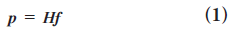
This formulation assumes that the PET data is deterministic, containing no statistical noise. Analytic reconstruction methods are based on this formulation. They provide a direct solution of f from p, and this simplified imaging model leads to relatively fast reconstruction techniques.

However, the PET data has an inherent stochastic nature. There are uncertainties associated with several aspects of PET physics, including: the positron decay process, the attenuation effects, the additive scatter and random events, and the photon detection process. These uncertainties can be modeled to yield more precise reconstructed images. In this regard, Equation 1 models only the average behavior of the imaging system, and a statistical formulation should be:

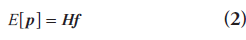
where E[•] denotes mathematical expectation. This formulation is used in most iterative reconstruction methods. As we will see later, modeling the data statistics can lead to improved reconstruction results.

2D versus fully 3D PET imaging

In 2D PET imaging, the data are only collected in direct and cross planes (Figure 4). A direct plane is perpendicular to the scanner axis, and a cross plane connects detector elements in two adjacent detector rings. 2D images are reconstructed on each of the planes, and are stacked to form a 3D image volume. So 2D PET imaging produces a 3D image volume.

In fully 3D imaging, coincidences are also recorded along the oblique planes (Figure 4). This permits better use of the emitted radiation, resulting in increased scanner sensitivity. For a given radiation dose and imaging time, fully 3D imaging typically leads to 5–10‑times more detected events [7,8]. This increased sensitivity can improve signal-to-noise performance in reconstructed images. But on the negative side, fully 3D measurements require much more data storage and reconstruction processing time, and contain significantly more scatter and random coincidence events than 2D data. These drawbacks hindered the use of fully 3D imaging in the early development of PET. With advances in data storage, computation speed and scatter correction [9,10], fully 3D imaging is now widely used clinically.

Quantitative corrections

To achieve quantitative imaging in which each image voxel value represents the true tissue activity concentration, a number of correction factors need to be estimated [11]. The measured coincidence events in prompt time window P are related to the true coincidence events T as:

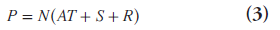
where A, R, S and N are the attenuation, random, scatter and normalization correction factors discussed below. These corrections can either be applied to the raw PET data, or they can be incorporated in iterative reconstruction methods.

Attenuation correction

When the emitted positron annihilates, it forms two photons each with an energy of 511 keV. When these two photons are detected at the same time, they are paired together as a true coincident event. At this photon energy, a large fraction of the emitted photons will interact in the subject before they exit the body. These interactions are dominated by Compton scattering, which reduces the photon energy and alters its direction. When a photon fails to travel along a straight line, due to scattering or other interactions, it is attenuated, representing the largest degradation to PET data. The probability of attenuation for a given pair of annihilation photons is independent of the position of the annihilation along the LOR, making it possible to precorrect for this effect.

Attenuation correction factors can be determined through direct measurements. A transmission scan is performed by using an external source of radiation that transmits photons through the body to the detector. A blank scan is also performed, and the ratio between the blank sinograms and the transmission sinograms are calculated as the attenuation correction factors [11,12]. The main drawback of this method is that the estimates are noisy for low activity transmission scans. Alternatively, the transmission data can be reconstructed into an image of attenuation coefficients through statistical methods [13].

Combined PET‑CT scanners provide another solution to this problem. A 511 keV attenuation map can be generated from the CT image. Multilinear scaling methods are used to convert attenuation coefficients measured with x‑ray CT (typically at 30–120 keV) to appropriate values at 511 keV. The correction factor for an individual sinogram element is calculated by integrating the attenuation coefficients along the corresponding LOR [14]. The use of CT for PET attenuation correction can lead to slight biases due to the approximate scaling of photon energies. On the other hand, CT-based attenuation correction produces attenuation correction factors with much lower noise, and at a much faster scan time, compared with conventional transmission scans [15]. Currently, CT-based attenuation correction is used with modern PET/CT scanners.

Once attenuation correction factors are determined for each sinogram element, they are applied as multiplicative correction factors either before reconstruction or during iterative reconstruction.

Scatter & random corrections

In PET imaging, the true coincidence data are contaminated by two types of additive physical effects, scatter and random coincidences. Scatter events refer to coincidence detection in which one or both photons have been scattered. The photon paths are not co-linear after scattering, and such events are incorrectly positioned. Although scatter events produce a fairly uniform error signal across the field of view, their contribution needs to be corrected for proper quantification. Most systems use some form of energy thresholding to discriminate heavily scattered photons from their 511 keV counterparts. Even with thresholding, additional correction techniques, such as simulated scatter models, are required. In these methods, images are first reconstructed without scatter correction, and the initial reconstruction, together with the attenuation map, is used to simulate scatter events [9,16,17].

Random events refer to the coincidence detection of two photons from separate annihilations. These events do not contain spatial information of annihilations, and will lead to reduced image contrast and image artifacts. There are two main methods for random event estimation. The first is to use a delayed time window, which contains purely random events and is an estimate of the random events in the prompt window [18,19]. The second method is to estimate random event rate from the singles counting rate for a given detector pair and coincidence time window. While these two methods can correct the mean of the data, the corrected data still have degraded variance due to the noise added by the random coincidences [20].

The scatter event and random event estimates are subtracted from the raw data, or the corrections can be incorporated in iterative reconstruction methods.

Detector efficiency correction & dead time correction

In a PET system, the coincidence detection efficiency varies between different pairs of detector elements, due to minor variations in detector material, electronics and geometry. Detector efficiency correction (‘normalization’) uses a multiplication factor to correct for these nonuniformities. The correction factors can be determined by collecting data from a uniform plane source or rotating rod source(s) of activity [21]. Another way is to factorize the efficiency of a detector pair as the product of individual detector efficiencies and geometrical factors, known as the component-based method [22,23]. These methods can provide low-variance estimates of normalization factors.

After receiving a photon, the detector has a time period in which it is ‘dead’ to new events. At a high counting rate, the dead time throughout the system can significantly limit the detection efficiency and the true system count rate will not increase linearly with activity in the field of view. Correction for dead time typically involves a model for the system dead time behavior at different count rate levels [24].

2D PET image reconstruction

Analytic image reconstruction

Analytic reconstruction methods assume that the PET data is noise-free, and attempt to find a direct mathematical solution for the image from known projections. A comprehensive review on the topic was given by Kinahan et al. [25].

Central section theorem & direct Fourier reconstruction

The central section theorem (also know as projection slice or central slice theorem) is the cornerstone of analytic image reconstruction. This theorem relates the projection data with the object activity distribution through a mathematical tool called the Fourier transform [26]. The 2D central section theorem states that the 1D Fourier transform of a projection at angle Ø is equivalent to a section at the same angle through the center of the 2D Fourier transform of the object:

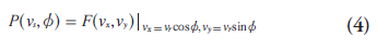
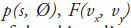where is the 1D Fourier transform of projection is the 2D Fourier transform of the object distribution f(x, y) and v_x is the Fourier domain conjugate for x.

Based on this theorem, direct Fourier methods have been proposed for image reconstruction. These methods take the 1D Fourier transform of each row in the sinogram (corresponding to one projection), and interpolate and sum the results on a 2D rectangular grid in Fourier domain. Then the inverse 2D Fourier transform is performed to obtain the image. The main difficulty in direct Fourier reconstruction is the interpolation involved. The reconstructed image strongly depends on the accuracy of interpolation, and is very sensitive to interpolation errors. While interpolation can be improved with different basis functions [27], direct Fourier methods are not as widely used as the filtered backprojection method, which is described next.

Filtered backprojection

Filtered backprojection is the most common method for analytic image reconstruction. It is also the most widely used method for CT image reconstruction. Its popularity arises from the combination of accuracy, speed of computation and simplicity of implementation. Details of the algorithm can be found in [26,28]. Here we describe the main components of the method.

An intuitive method of image reconstruction is backprojection, which is the adjoint to the forward projection process of data acquisition. The counts from a detector pair are projected back into an image array along the LOR adjoining that detector pair. Since the original image activity values at each location are lost in the forward projection, we place a constant value into all pixels along the LOR. By repeating this for all detector pairs, we obtain a linear superposition of backprojections.

Straight backprojection returns an image resembling the true activity distribution, but it is a blurred version of the object, since counts are distributed equally along the LORs. Mathematical derivations show that the 2D Fourier transform of the backprojection is the 2D Fourier transform of the object weighted by the inverse distance from the origin [26]:

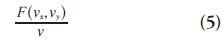
and the weighting term

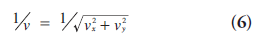
amplifies low frequencies and attenuates high frequencies, leading to the blurred reconstruction result.

Additional steps are needed to compensate for the blurring in direct backprojection. The most straightforward method is the backprojection filtering reconstruction. The projection data is first backprojected, and then filtered in Fourier space with the cone filter v, and finally inverse Fourier transformed. The disadvantage of backprojection filtering is the computation redundancy in the backprojection step (backprojection needs to be computed on a larger image matrix than the final result) [25]. To avoid this, the filtering and backprojection steps are interchanged, leading to the standard filtered-backprojection (FBP) method. The implementation of FBP reconstruction can be summarized as follows. For each projection angle:

• Take the 1D Fourier transform of the projection

• In the Fourier domain, filter the projection with a ramp filter |vs| (a section through the rotationally symmetric 2D cone filter, v)

• Take inverse Fourier transform to obtain the filtered projection

• Backproject the filtered projection

Noise control

In practice, the ramp filter |v_s| needs to be modified to control the noise level in reconstructed images. Photon detection is a random counting process, with a high level of noise due to limited photon counts. The ramp filter amplifies highfrequency components, which are dominated by noise, leading to very noisy reconstructions. One solution is to modify the ramp filter with a low-pass filter, leading to filters that are similar to the ramp filter at low frequencies but have reduced amplitude at high frequencies. The reconstructed image will have a reduced noise level, at the expense of degraded image resolution. Typical choices are Hann filters or Shepp– Logan filters [25]. By varying the cutoff frequency of the filters, one can obtain the desired tradeoff between noise level and spatial resolution (Figure 5). The noise in reconstructed images is controlled at the expense of resolution. Ideally, the tradeoff between noise and resolution should be adjusted to optimize the clinical task at hand.

Limitations of analytic image reconstruction methods

While analytic reconstruction methods, in particular the FBP algorithm, are fast and easy to implement, the reconstruction accuracy is limited by several factors. First, analytic image reconstruction cannot model the degrading factors in a PET scanner, such as intercrystal scatter, positron range and noncollinearity. Second, these methods take no account of the stochastic variability in photon detection.

Iterative image reconstruction

Modeling the statistical noise of PET data and the physical effects of the imaging model can lead to improved performance over the analytical methods. The improvement, however, comes at the expense of increased complexity of the reconstruction problem, making it impossible to obtain a direct analytic solution. Consequently, the reconstruction problem is solved iteratively, meaning the image estimate is progressively updated towards an improved solution. Initially, the computation cost hindered iterative reconstruction’s clinical use, but advances in computation speed and the development of efficient algorithms have permitted widespread clinical use of iterative image reconstruction methods [6,29–31].

Formulation of iterative methods

The basic concept of iterative reconstruction is summarized here. First, we make an initial estimate of the object activity distribution. Then we calculate the estimated projection by forward projecting the initial estimate. Based on the comparison between estimated and measured projections, the initial estimate is adjusted according to certain criterion. This ‘forward project, compare, backproject, adjust’ procedure is repeated till the estimated image reaches a desired solution.

All iterative methods can be characterized with two key components. First, a criterion that defines the ‘best’ image. This criterion is represented as an objective (or cost) function, which measures the similarity (or difference) between the image estimate and the best image. The most widely used criterion is the maximum likelihood (ML) approach, which will be discussed in detail later. Another common criterion is the least square principle, which measures the difference between measured and estimated projections using Euclidean distance [32]. Second, all iterative methods require a numerical algorithm to determine how the image estimate should be updated at each iteration based on the criterion. The expectation-maximization (EM) algorithm is commonly used to find the ML image estimate, and the classic MLEM algorithm will be discussed.

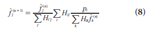
Historically, much research effort has concentrated on these two components: designing the optimization criterion and developing efficient algorithms. However, there are three other key factors that strongly influence the reconstruction result. These three factors need to be carefully selected to obtain a desired image estimate. First, the image representation specifies a model for the image. The most common one is using distinct pixels (2D image elements) or voxels (3D image elements) to discretize the image domain. Alternative methods have been proposed. One example are ‘blobs’, which have spherical symmetry and bell-shaped radial profiles [27,33]. Second, the imaging model describes the physics of the measurement process. It relates the image to the data. The imaging matrix H in Equation 2 is such a model, where each element H_ij contains the probability that image element f_j contributes to data element pi. It can model only the geometrical mapping from the object to the data, or it can include other physical effects such as attenuation and detector blurring. For the latter, the imaging matrix can be factorized as:

with each matrix representing one physical component [30,34,35]. Third, the statistical model describes the uncertainty of PET measurements (i.e., the probability distribution of measurements around their mean values). Since photon detections are Poisson distributed, most methods adopt a Poisson model. However, the measurement distribution may be changed by data correction steps as described previously, so other models have been proposed (e.g., shifted Poisson model [36]) to describe the data statistics more accurately.

Different choices in these three components, together with variations in the criterion and the algorithm, have resulted in a great variety of iterative reconstruction methods [6,29,30]. We will focus on the two most representative methods in the following discussion, and then briefly review other types of iterative reconstruction.

MLEM method

Maximum-likelihood estimation is a standard statistical estimation method. It produces an estimate that maximizes the likelihood function (i.e., the estimate that ‘most likely’ leads to the measured data). The EM algorithm is an efficient algorithm to find the ML estimate. MLEM image reconstruction provides the foundation for many popular iterative methods. It adopts ML as the optimization criterion, and uses the EM algorithm to find the optimal solution.

The EM algorithm, first described in detail by Dempster et al. [37], is a numerical algorithm to solve incomplete data problems in statistics. This general algorithm was later introduced to emission tomographic reconstruction [38,39]. For image reconstruction with a Poisson likelihood, the MLEM method is a simple iterative equation:

where is the image estimate for voxel j at iteration n. The flow of the algorithm is shown in Figure 6. The initial guess (often a blank or uniform grayscale image) is forward projected into the projection domain (denominator on right side). Then, the comparison between estimated and measured projections is determined by calculating their ratio. This ratio in projection domain is backprojected to the image domain and properly weighted, providing a correction term. Finally the current image estimate is multiplied by the correction term, generating the new estimate This process is repeated and the image estimate converges to the ML solution.

While the MLEM algorithm has consistent and predictable convergence behavior, it suffers from two main drawbacks. First, the method yields very noisy images due to the ill-conditioning of the problem [39]. One common solution is stopping the algorithm before convergence, and several stopping rules have been proposed [40,41]. Another solution is to apply a smoothing filter to the reconstructed image for noise suppression [42]. Likewise, sieves (an operation that suppresses high frequency noise) can be applied during each iteration to impose smoothness [43]. These solutions reduce the noise at the expense of increasing bias.

The second drawback of MLEM is its slow convergence. While the algorithm is stopped early in practice, it typically requires many iterations (in the order of 30–100 iterations with typical PET data) to reach an acceptable solution. Since each iteration involves forward and backward projections, and FBP reconstruction is equivalent to one backprojection, MLEM methods require considerably more computation time than FBP methods.

Ordered subsets methods: ordered subsets EM

To address the issue of slow convergence, different methods have been proposed to accelerate MLEM. Several researchers reformulated the update equation to increase the magnitude of change at each iteration [44,45], and others proposed to update each pixel individually in a space-alternating generalized EM algorithm [46]. A larger category of methods, of which ordered subsets EM (OSEM) is the most popular, uses only part of the data at each update [47–49].

The OSEM algorithm [47] partitions the projection data into B subsets (typically mutually exclusive) and uses only one subset of data S_b for each update. It results in a slight modification of the update equation:

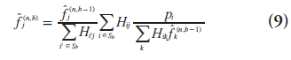
where b is the index for subiteration (i.e., update with one subset of data), and Each pass of the entire data set involves a greater number of updates, leading to significant acceleration compared with MLEM. The number of subsets determines the degree of acceleration. In practice, OSEM converges roughly B times faster than MLEM. Figure 7 shows OSEM reconstruction at different iterations with a different number of subsets. Note that the result at iteration one with ten subsets is similar to the result at iteration ten with one subset, indicating that MLEM (i.e., OSEM with one subset) needs approximately ten‑times the computation time of ten‑subset OSEM to achieve a similar reconstruction result.

One drawback of OSEM is that it is not guaranteed to converge to the ML solution. As with the MLEM method, due to the increasing noise level with iterations, the algorithm is terminated early and/or the reconstructed image is postsmoothed (Figure 8). Other variants of the subset-based methods include rescaled blockiterative EM algorithm [49] and the row-action ML algorithm [48], which are shown to converge to the ML solution under certain conditions. However, OSEM is currently the most widely use iterative reconstruction method.

Other iterative methods

So far we have discussed the MLEM method and its variant, the OSEM algorithm. Now we will briefly review several other types of iterative methods.

Algebraic reconstruction techniques (ART) enjoyed considerable interest in the early development of emission tomography. ART reconstruction attempts to find an image that satisfies a set of known constraints. These constraints are determined by the PET data and/or prior knowledge of the image (e.g., non-negative pixel activity) [28]. The ART problem is solved iteratively and block-iterative (or ordered subset) methods are available to accelerate the convergence [50,51]. The main limitation of ART is that it does not model the statistics of PET data, leading to complications in the presence of statistical noise. In emission tomography reconstruction, ART methods have been replaced by ML-based statistical methods (e.g., MLEM, OSEM).

In addition to specifying how well the image estimate fits the data (e.g., using the ML criterion), one can also include desired image properties (e.g., smoothness, non-negativity) in the optimization criterion. In essence, ML methods assume a statistical model for the data. By incorporating both a statistical model for the data and the image, one arrives at the formulation of maximum a posteriori (MAP) reconstruction. Instead of maximizing the likelihood function, the algorithm seeks to maximize the posterior probability density, so that an a priori model of the image distribution is enforced in the reconstruction. The a priori knowledge, or ‘prior’, is often a smoothness constraint [46,52], which enforces a more elegant noise control method than early termination of algorithm. The priors may also include anatomical information from other imaging modalities such as CT or MRI [53,54]. The MAP solution can be computed using generalizations of the EM algorithm [52,55,56], and ordered subset methods can be applied to speed up MAP reconstruction [57,58]. Challenges of MAP methods include determination of the desired magnitude of the influence of the prior and the additional computational demand of enforcing this prior information.

The priors in MAP reconstruction can be considered as a penalty on solutions to enforce desirable properties, so MAP methods are sometimes called penalized ML methods. This penalization formulation can be extended to the traditional least square methods. One representative method is the penalized weighted least square algorithm [59,60], which is equivalent to the MAP method with a Gaussian likelihood model under certain conditions of the data variance terms [61].

3D PET image reconstruction

Fully 3D PET data

Fully 3D PET imaging acquires data from both transverse and oblique imaging planes, offering increased scanner sensitivity and potentially improved signal-to-noise performance. Fully 3D PET data differs from its 2D counterpart in two aspects: spatially-varying scanner response and data redundancy. In 2D imaging, the detectors are rotationally symmetric, so the projections are available at all angles in the imaging plane. The 3D analog would be a spherical scanner with detectors surrounding the object, which is unrealistic in practice. Since most PET scanners have a cylindrical geometry, projections are truncated in the axial direction due to the limited axial length of scanner, resulting in a spatial variance in scanner response. The observed intensity of a point source will vary depending on the position of the point source in the scanner’s field of view, causing complications for analytic image reconstruction [25].

The second feature of 3D PET data is its redundancy. Recall in 2D imaging, a 3D image volume is reconstructed by stacking reconstructed images from each of the transverse 2D sinograms. So the set of 2D sinograms alone contains sufficient information to reconstruct the 3D image volume. In this sense, fully 3D PET data, which contains detections from both transverse and oblique planes, has an inherent redundancy. This redundancy can be utilized to improve the signal-to-noise performance. And as we will discuss later, this feature also provides a solution for 3D analytic reconstruction.

Rebinning methods

An intuitive solution to 3D PET reconstruction is to convert the 3D data to decoupled sets of 2D data and apply 2D reconstruction strategies. This conversion involves some form of signal averaging, and the process is called ‘rebinning’.

The most straightforward rebinning method is single-slice rebinning [62]. It calculates the average axial position of a coincidence event, and places the event in the sinogram closest to that average position. This method is fast and efficient, but it also causes blurring in the axial direction.

A more accurate method is the Fourier rebinning (FORE) algorithm. The details of FORE are beyond the scope of this article and we refer interested readers to [63]. In principle, FORE relates the Fourier transform of oblique sinograms to the Fourier transform of transverse sinograms. This approximate relation converts the oblique sinograms into a set of equivalent transverse sinograms. Compared with single-slice rebinning, FORE slightly amplifies statistical noise, but leads to significantly less distortion [64]. Similar rebinning methods include FOREX [63,65] and FORE-J [66], and their relation to FORE is discussed in [66].

Rebinning methods decompose the 3D reconstruction problem into a set of 2D problems. This greatly reduces the data storage and computation requirements. More importantly, the rebinned 3D PET data can be reconstructed using either analytic or iterative 2D reconstruction methods. The limitation of rebinning methods is that they lead to spatial distortion or noise amplification.

3D analytic reconstruction

Conceptually, the FBP method can be extended to 3D reconstruction. However, as discussed in the ‘Fully 3D PET data’ section, the spatial variance of 3D PET data complicates the analytic reconstruction. For example, since projections are truncated in the axial direction, it is not possible to compute the Fourier transform of projections by simply using the fast Fourier transform algorithm.

The most representative 3D analytic reconstruction method is the 3D reprojection algorithm [67]. It restores the spatial invariance by making use of the data redundancy. Transverse sinograms are extracted from the 3D data and reconstructed with 2D FBP. Reconstructed images are stacked into a 3D image volume, which is then reprojected into the projection domain. In this way, the unmeasured regions of projections are estimated, and 3D FBP method can be used for reconstruction. Further details of implementation can be found in [68].

Compared with 2D FBP reconstruction, 3D reprojection algorithm can significantly improve the signal-to-noise performance. This potentially allows a higher spatial resolution in reconstructed images, since a higher cutoff frequency can be used in the reconstruction filter.

3D iterative image reconstruction

Iterative reconstruction methods can be directly adapted to 3D PET data, although the computation complexity for the imaging model H increases dramatically. Iterative methods can include the spatial variance of the 3D data in the imaging model, so no additional steps are required as in analytic 3D image reconstruction. For 3D PET, the object is represented by a set of voxels rather than 2D pixels, and the imaging model relates the voxel activity to the 3D projections.

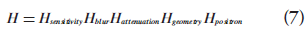
The major challenge for fully 3D iterative reconstruction is the computational demand. The imaging model H becomes extremely large due to the added dimensionality in both the image and the projection domains. These increases require more data storage space and more computation time. One useful tool is the factorized system model [30,34,35], as shown in Equation 7. Advances in computer processing and faster algorithms are helping to overcome these challenges.

Current developments & challenges

Selection of image reconstruction parameters

One challenge in image reconstruction is the selection of proper reconstruction parameters. In analytic reconstruction, the roll-off and cutoff frequencies of the reconstruction filter (e.g., Hann filter) will determine the noise–resolution tradeoff. More reconstruction parameters are involved with iterative reconstruction. We present examples in Figures 7 & 8 of how the choice of iteration, number of subsets and postsmoothing can affect the final image. Commercial scanners typically provide the option for end users to change these parameters. For OSEM-type reconstruction, the optimal set of parameters would be object-dependent. The reconstruction parameters should be optimized for a given detection or quantification task. Evaluation is still ongoing to study how different parameters affect figures- of-merit of the reconstructed images.

Incorporation of anatomical information

PET imaging has relatively low resolution compared with anatomical imaging modalities such as CT and MRI. PET/CT scanners offer the advantage of anatomical information (from the CT image) that can be incorporated into PET image reconstruction. Such anatomical information can guide PET image reconstruction and noise regularization, leading to improved image quality in terms of signal-to-noise ratio and quantitative accuracy in PET images (Figure 9) [53,54,69,70]. Several studies have applied anatomical information in a postprocessing step [71,72]. There is a clearer link with the imaging physics, however, if the anatomical information is integrated within an image reconstruction (e.g., MAP) framework [53,54,69,70,73]. Typically, these techniques require that the anatomical image must first be segmented to provide the boundary information. However, segmenting the CT image is a potentially difficult problem in practice. Methods requiring little or no segmentation have also been proposed, and one approach is using mutual information to define the anatomical priors [74,75]. Another challenge is the registration of the two image modalities. While PET/CT scanners allow the acquisition of functional and anatomical information in the same session, physiologic motions (e.g., cardiac and respiratory motions) can cause artifacts in the fused image [76,77]. These issues should be properly considered when incorporating anatomical information into image reconstruction [78,79], and the challenges listed above have hampered adoption of such methods.

TOF imaging

TOF imaging was originally proposed in the early development of PET scanners in the 1980s. By measuring the arrival time difference of the two annihilation photons in the detectors, TOF imaging can attempt to position the annihilation location along the line of response. This TOF positioning requires exceptionally fast timing and can lead to improved signal-to-noise performance in the reconstructed images [80,81]. TOF PET was extensively studied in the 1980s, but sufficient timing resolution and detector efficiency could not be achieved to provide image quality improvement. Recent instrumentation advances have renewed the development of TOF imaging and made clinical TOF PET a reality [82]. Studies have shown that TOF imaging can provide improved contrast-to-noise (Figure 10) [83] and lesion detectability [84] in clinical PET. Further evaluation of the benefits of TOF imaging in clinical PET is still needed.

Point spread function modeling

The performance of iterative image reconstruction methods can be further improved when the full physics of the imaging process is accurately and precisely modeled. One important component of the physics modeling is the detector point spread function (PSF). Detector PSF in projection data space can be obtained through analytical derivations [85,86], Monte Carlo simulations [35,87] or experimental measurements [88,89]. Alternatively, the resolution modeling can be performed in the reconstructed image space [90,91]. Including the PSF model in reconstruction methods has been shown to improve the spatial resolution in the reconstructed images (Figure 11) [87,88]. PSF modeling can also lead to improved contrast recovery [92,93] and lesion detectability [94]. However, there is a growing recognition that PSF-based reconstruction results have different noise properties [92] and may contain quantitation errors (e.g., overshoot at object edges, often referred to as the Gibbs effect) [89], which is still under evaluation.

Motion correction

Considering that data for a single PET imaging field of view is often acquired over 2–5 min, patient motion during imaging can affect both the detection and quantitation performance of PET. Proper strategies are needed to correct large-scale patient motion (e.g., head motion), cardiac motion and respiratory motion. Head motion is assumed to be rigid (i.e., consisting of translational and rotational transformations only). Correction methods include registering images obtained at different frames [95], or using forward-projected data for motion detection [96]. An alternative approach is to correct motion effects in a postprocessing step, by using deconvolution algorithms [97]. Compensation for nonrigid cardiac and respiratory motion typically involves gating methods, with each gated frame representing a particular cardiac or respiratory cycle (Figure 12) [98]. One correction method is a two-step solution: initial motion estimation from gated images (without motion correction in reconstruction), followed by a refined reconstruction including the motion information [99]. An alternative approach is to estimate the motion within the reconstruction step [100,101].

4D dynamic/parametric reconstruction

Dynamic PET imaging can be performed through a sequence of contiguous acquisitions, or list-mode acquisition followed by the specification of timing frames, all leading to a 4D data set. List-mode acquisition records the detection time of each coincidence event in addition to its spatial coordinates. By appropriate data regrouping, list mode data can be reformatted to a sequence of temporal frames. The image of radioactivity distribution at each temporal frame can be reconstructed, producing an estimate of the changing activity over time. Then with tracer kinetic models, the set of reconstructed activity images can be used to estimate physiological parameters of interest (e.g., metabolic rate, tissue perfusion) for a selected region or each voxel [102]. Conventionally, the spatial distribution is reconstructed independently for each imaging frame. This frame-by-frame approach, however, fails to explore the temporal information of dynamic data, and leads to noisy reconstruction due to the low signal-to-noise ratio of data. A more precise way is to perform image or kinetic parameter reconstruction from the 4D data set, by including certain temporal modeling in reconstruction. Smooth temporal basis functions can be used to constrain the possible choices of time activity curves [103–105]. Principle component analysis can be used to transform the dynamic PET data into decorrelated sets, allowing fast reconstruction [106]. Several approaches also attempt to reconstruct parametric images directly from PET data [107]. These review articles provide broader and more detailed discussions on this topic [108,109].

Reconstruction for application-specific scanners

Since the 1990s, advances in instrumentation [110] and reconstruction algorithms [35,111] have improved the spatial resolution of PET. These advances have permitted the application of PET to the imaging of small animals (mice and rats), which are invaluable models of human disease. Small animal PET imaging has permitted rapid testing of new drugs [112] and improved understanding of gene expression [113]. Interested readers are referred to these review articles for comprehensive discussions on small animal PET instrumentation and methodology [114,115]. In general, these systems offer interesting challenges to image reconstruction because they require high-resolution performance and often contain novel geometries, such as systems with large detector gaps or rotating gantries.

The combination of PET and MRI is currently an active research area. MRI provides structural images with high spatial resolution and excellent soft tissue contrast. An integrated MRI/PET scanner could allow simultaneous acquisitions of the two imaging modalities in a fixed geometry, by building a PET insert into existing MRI scanners or adopting novel MRI scanner designs [116]. These systems provide aligned high-resolution MRI images, which can be used as anatomical priors for PET image reconstruction and facilitate precise localization of PET signals. The integrated MRI/PET scanner will likely generate new opportunities: for example, imaging two molecular targets with distinct MRI and PET imaging probes [117]. One challenge of the integrated system is the interferences between the two modalities, which should be minimized to achieve consistent performance with standalone PET or MRI devices. Another challenge is attenuation correction of PET data using MRI images, which is beyond the scope of this article. Details of integrated MRI/PET systems are presented in these review articles [116–119].

Future perspective

PET image reconstruction is a well-researched yet actively evolving field. In addition to the challenges discussed above (TOF imaging, improved system modeling, motion correction and dynamic imaging), there are other ongoing efforts in this area. There is a growing need for more accurate quantitation of PET. For example, tumor metabolism via FDG-PET/CT can be used as a biomarker, which should be accurate and reproducible in multicenter, multivendor clinical trials and meta-analyses. Additional efforts are required to develop clinically viable image reconstruction techniques that provide accurate, precise quantitative estimates of tracer distribution, independent of feature size, shape and location. Improved quantitative image reconstruction, together with other advances in instrumentation and data processing, could enhance the use of PET/CT imaging in patient care and in clinical studies of pathophysiology and therapeutic interventions [120].

Financial & competing interests disclosure

This work is supported by NIH grants HL086713, CA74135 and CA115870, and by a grant from GE Healthcare. The authors have no other relevant affiliations or financial involvement with any organization or entity with a financial interest in or financial conflict with the subject matter or materials discussed in the manuscript apart from those disclosed.

No writing assistance was utilized in the production of this manuscript.

Papers of special note have been highlighted as:
* of considerable interest

References

1. Bailey D, Townsend D, Valk PE et al.: Positron Emission Tomography: Basic Sciences. Springer, London, UK (2005).
2. Phelps ME: PET: Molecular Imaging and Its Biological Applications. Springer, London, UK (2004).
3. Weber WA, Figlin R: Monitoring cancer treatment with PET/CT: does it make a difference? J. Nucl. Med. 48(1), 36S–44S (2007).
4. Weber WA: Use of PET for monitoring cancer therapy and for predicting outcome. J. Nucl. Med. 46(6), 983–995 (2005).
5. Sorenson JA, Phelps ME: Physics in Nuclear Medicine. Grune & Stratton, FL, USA (1987).
6. Lewitt RM, Matej S: Overview of methods for image reconstruction from projections in emission computed tomography. Proc. IEEE 91(10), 1588–1611 (2003). & Overview of image reconstruction methods for emission tomography.
7. Cherry SR, Dahlbom M, Hoffman EJ: 3D PET using a conventional multislice tomograph without septa. J. Comput. Assist. Tomogr. 15(4), 655–668 (1991).
8. Townsend DW, Geissbühler A, Defrise M et al.: Fully three-dimensional reconstruction for a PET camera with retractable septa. IEEE Trans. Med. Imag. 10(4), 505–512 (1991).
9. Ollinger JM: Model-based scatter correction for fully 3D PET. Phys. Med. Biol. 41(1), 153–176 (1996).
10. Wollenweber SD: Parameterization of a model-based 3D PET scatter correction. IEEE Trans. Nucl. Sci. 49(3), 722–727 (2002).
11. Lewellen TK, Karp JS: PET systems. In: Emission Tomography: The Fundamentals of PET and SPECT. Wernick M, Avarsvold J (Eds). Elsevier, CA, USA, 169–178 (2004).
12. Bailey DL: Transmission scanning in emission tomography. Eur. J. Nucl. Med. 25(7), 774–787 (1998).
13. Fessler JA: Statistical image reconstruction methods for transmission tomography. In: Handbook of Medical Imaging: Vol. 2 Medical Image Processing and Analysis. Sonka M, Fitzpatrick JM (Eds). SPIE, FL, USA, 1–70 (2000).
14. Kinahan PE, Townsend DW, Beyer T et al.: Attenuation correction for a combined 3D PET/CT scanner. Med. Phys. 25(10), 2046–2053 (1998).
15. Kinahan PE, Hasegawa BH, Beyer T: X-ray based attenuation correction for PET/CT scanners. Semin. Nucl. Med. 33(3), 166–179 (2003).
16. Watson C, Newport D, Casey ME: Evaluation of simulation-based scatter correction for 3D PET cardiac imaging. IEEE Trans. Nucl. Sci. 44, 90–97 (1997).
17. Holdsworth CH, Levin CS, Farquhar TH et al.: Investigation of accelerated Monte Carlo techniques for PET simulation and 3D PET scatter correction. IEEE Trans. Nucl. Sci. 48(1), 74–81 (2001).
18. Brasse D, Kinahan PE, Lartizien C et al.: Correction methods for random coincidences in fully 3D whole-body PET: impact on data and image quality. J. Nucl. Med. 46(5), 859–867 (2005).
19. Williams CW, Crabtree MC, Burgiss SG: Design and performance characteristics of a positron emission computed axial tomograph: ECAT-II. IEEE Trans. Nucl. Sci. 26(1), 619–627 (1979).
20. Stearns CW, McDaniel DL, Kohlmyer SG et al.: Random coincidence estimation from single event rates on the Discovery ST PET/ CT scanner. Proceedings of the 2003 IEEE Nuclear Science Symposium and Medical Imaging Conference. Portland, OR, USA, 19–25 October, 5, 3067–3069 (2003).
21. Hoffman EJ, Guerrero TM, Germano G et al.: PET system calibrations and corrections for quantitative and spatially accurate images. IEEE Trans. Nucl. Sci. 36(1), 1108–1112 (1989).
22. Defrise M, Townsend DW, Bailey D et al.: A normalization technique for 3D PET data. Phys. Med. Biol. 36(7), 939–952 (1991).
23. Casey ME, Gadagkar H, Newport D: A component based method for normalization in volume PET. Presented at: Third International Meeting on Fully Three- Dimensional Image Reconstruction in Radiology and Nuclear Medicine. Domaine d’Aix- Marlioz, Aix-les-Bains, France, 4–6 July 1995.
24. Germano G, Hoffman EJ: Investigation of count rate and dead time characteristics of a high resolution PET system. J. Comput. Assist. Tomogr. 12(5), 836–846 (1988).
25. Kinahan P, Defrise M, Clackdoyle R: Analytic image reconstruction methods. In: Emission Tomography: The Fundamentals of PET and SPECT. Wernick M, Avarsvold J (Eds). Elsevier, London, UK, 421–442 (2004). & Discusses analytic image reconstruction in detail.
26. Kak AC, Slaney M: Principles of Computerized Tomographic Imaging. IEEE Press, NY, USA (1988). & Discusses the mathematical principles of tomographic imaging and image reconstruction.
27. Lewitt RM: Alternatives to voxels for image representation in iterative reconstruction algorithms. Phys. Med. Biol. 37(3), 705–716 (1992).
28. Herman GT: Image Reconstruction from Projections. Academic Press, NY, USA (1980).
29. Lalush DS, Wernick MN: Iterative image reconstruction. In: Emission Tomography: The Fundamentals of PET and SPECT. Wernick M, Avarsvold J (Eds). Elsevier, London, UK, 443–472 (2004). & Comprehensive overview on iterative image reconstruction methods.
30. Leahy R, Qi J: Statistical approaches in quantitative positron emission tomography. Stat. Comput. 10(2), 147–165 (2000). & Survey on statistical image reconstruction methods.
31. Meikle SR, Hutton BF, Bailey D et al.: Accelerated EM reconstruction for total-body PET: potential for improving tumor detectability. Phys. Med. Biol. 39(10), 1689–1704 (1994).
32. Kay SM: Fundamentals of Statistical Signal Processing: Estimation Theory. Prentice Hall, NY, USA (1993).
33. Lewitt RM: Multidimensional digital image representations using generalized Kaiser– Bessel window functions. J. Opt. Soc. Am. A. 7(10), 1834–1846 (1990).
34. Qi J, Leahy RM, Hsu C et al.: Fully 3D Bayesian image reconstruction for the ECAT EXAT HR+. IEEE Trans. Nucl. Sci. 45, 1096–1103 (1998).
35. Qi J, Leahy RM, Cherry SR et al.: High resolution 3D Bayesian image reconstruction using the small animal microPET scanner. Phys. Med. Biol. 43, 1001–1013 (1998).
36. Yavuz M, Fessler JA: Penalized-likelihood estimators and noise analysis for randomsprecorrected PET transmission scans. IEEE Trans. Med. Imag. 18(8), 665–674 (1999).
37. Dempster A, Laird N, Rubin D: Maximum likelihood from incomplete data via the EM algorithm. J. R. Stat. Soc. 39(1), 1–28 (1977).
38. Lange K, Carson R: EM reconstruction algorithms for emission and transmission tomography. J. Comput. Assist. Tomogr. 8(2), 306–316 (1984).
39. Shepp LA, Vardi Y: Maximum likelihood reconstruction for emission tomography. IEEE Trans. Med. Imag. 2, 113–119 (1982).
40. Veklerov E, Llacer J: Stopping rule for the MLE algorithm based on statistical hypothesis testing. IEEE Trans. Med. Imag. 6(4), 313–319 (1987).
41. Johnson VE: A note on stopping rules on EM-ML reconstructions of ECT images. IEEE Trans. Med. Imag. 13(3), 569–571 (1994).
42. Llacer J, Veklerov E, Baxter LR et al.: Results of clinical receiver operating characteristics study comparing filtered backprojection and maximum likelihood estimator images in FDG PET studies. J. Nucl. Med. 34, 1198–1203 (1993).
43. Snyder D, Miller MP: The use of sieves to stabilize images produced with the EM algorithm for emission tomography. IEEE Trans. Nucl. Sci. 32(5), 3864–3872 (1985).
44. Lewitt RM, Muehllehner G: Accelerated iterative reconstruction for positron emission tomography based on the EM algorithm for maximum likelihood estimation. IEEE Trans. Med. Imag. 5(1), 16–22 (1986).
45. Kaufman L: Implementing and accelerating the EM algorithm for positron emission tomography. IEEE Trans. Med. Imag. 6(1), 37–51 (1987).
46. Fessler JA, Hero AO: Penalized maximumlikelihood image reconstruction using space-alternating generalized EM algorithms. IEEE Trans. Image Process. 4(10), 1417–1429 (1995).
47. Hudson H, Larkin R: Accelerated image reconstruction using ordered subsets of projection data. IEEE Trans. Med. Imag. 13, 601–609 (1994).
48. Browne JA, De Pierro AR: A row-action alternative to the EM algorithm for maximizing likelihoods in emission tomography. IEEE Trans. Med. Imag. 15, 687–699 (1996).
49. Byrne C: Block-iterative methods for image reconstruction from projections. IEEE Trans. Image Process. 5(5), 792–794 (1996).
50. Herman GT, Meyer LB: Algebraic reconstruction techniques can be made computationally efficient. IEEE Trans. Med. Imag. 12, 600–609 (1993).
51. Censor Y, Herman GT: On some optimization techniques in image reconstruction from projections. Appl. Numer. Math. 3(5), 365–391 (1987).
52. Hebert T, Leahy RM: A generalized EM algorithm for 3-D Bayesian reconstruction for Poisson data using Gibbs priors. IEEE Trans. Med. Imag. 8(2), 194–202 (1989).
53. Bowsher JE, Johnson VE, Turkington TG et al.: Bayesian reconstruction and use of anatomical a priori information for emission tomography. IEEE Trans. Med. Imag. 15(5), 673–686 (1996).
54. Gindi G, Lee M, Rangarajan A et al.: Bayesian reconstruction of functional images using anatomical information as priors. IEEE Trans. Med. Imag. 12, 670–680 (1993).
55. De Pierro AR: A modified expectation maximization algorithm for penalized likelihood estimation in emission tomography. IEEE Trans. Med. Imag. 14(1), 132–137 (1995).
56. Green PJ: Bayesian reconstruction for emission tomography data using a modified EM algorithm. IEEE Trans. Med. Imag. 9(1), 84–93 (1990).
57. De Pierro AR, Yamagishi M: Fast EM-like methods for maximum a posteriori estimates in emission tomography. IEEE Trans. Med. Imag. 20(4), 280–288 (2001).
58. Lalush DS, Frey EC, Tsui BMW: Fast maximum entropy approximations in SPECT using the RBI-MAP algorithm. IEEE Trans. Med. Imag. 19(4), 286–294 (2000).
59. Fessler JA: Penalized weighted least squares image reconstruction for positron emission tomography. IEEE Trans. Med. Imag. 13(2), 290–300 (1994).
60. Kaufman L: Maximum likelihood, least squares, and penalized least squares for PET. IEEE Trans. Med. Imag. 12(2), 200–214 (1993).
61. Lalush D, Tsui B: A fast and stable maximum a posteriori conjugate gradient reconstruction algorithm. Med. Phys. 22(8), 1273–1284 (1995).
62. Daube-Witherspoon ME, Muehllehner G: Treatment of axial data in three-dimensional PET. J. Nucl. Med. 28, 1717–1724 (1987).
63. Defrise M, Kinahan PE, Townsend DW et al.: Exact and approximate rebinning algorithms for 3-D PET data. IEEE Trans. Med. Imag. 16(2), 145–158 (1997).
64. Matej S, Karp JS, Lewitt RM et al.: Performance of the Fourier rebinning algorithm for PET with large acceptance angles. Phys. Med. Biol. 43, 787–795 (1998).
65. Liu X, Defrise M, Michel C et al.: Exact rebinning methods for three-dimensional PET. IEEE Trans. Med. Imag. 18(8), 657–664 (1999).
66. Defrise M, Liu X: A fast rebinning algorithm for 3D positron emission tomography using John’s equation. Inverse Probl. 15, 1047–1065 (1999).
67. Kinahan PE, Rogers JG: Analytic 3D image reconstruction using all detected events. IEEE Trans. Nucl. Sci. 36, 964–968 (1989).
68. Defrise M, Kinahan PE: Data acquisition and image reconstruction for 3D PET. In: The Theory and Practice of 3D PET 32. Townsend DW, Bendriem B (Eds). Kluwer Academic Publishers, Dordrecht, The Netherlands, 11–54 (1998).
69. Fessler JA, Clinthorne NH, Rogers WL: Regularized emission image reconstruction using imperfect side information. IEEE Trans. Nucl. Sci. 39(5), 1464–1471 (1992).
70. Comtat C, Kinahan PE, Fessler JA et al.: Clinically feasible reconstruction of 3D whole-body PET/CT data using blurred anatomical labels. Phys. Med. Biol. 47, 1–20 (2002).
71. Cheng PM, Kinahan PE, Alessio A et al.: Post-reconstruction partial volume correction in PET/CT imaging using CT information. Presented at: Radiological Society of North America. Chicago, IL, USA, 28 November– 3 December 2004 (Abstract 371).
72. Boussion N, Hatt M, Lamare F et al.: A multiresolution image based approach for correction of partial volume effects in emission tomography. Phys. Med. Biol. 51(7), 1857–1876 (2006).
73. Alessio A, Kinahan P: Improved quantitation for PET/CT image reconstruction with system modeling and anatomical priors. Med. Phys. 33, 4095–4103 (2006).
74. Rangarajan A, Hsiao IT, Gindi G: A Bayesian joint mixture framework for the integration of anatomical information in functional image reconstruction. J. Math. Imaging Vis. 12, 199–217 (2000).
75. Somayajula S, Asma E, Leahy R: PET image reconstruction using anatomical information through mutual information based priors. Nuclear Science Symposium Conference Record 2722–2726 (2005).
76. Cohade C, Osman M, Marshall LT et al.: PET/CT: accuracy of PET and CT spatial registration of lung lesions. Eur. J. Nucl. Med. 30, 721–726 (2003).
77. Osman M, Cohade C, Nakamoto Y et al.: Clinically significant inaccurate localization of lesions with PET/CT: frequency in 300 patients. J. Nucl. Med. 44, 240–243 (2003).
78. Camara O, Delso G, Colliot O et al.: Explicit incorporation of prior anatomical information into a nonrigid registration of thoracic and abdominal CT and 18-FDG whole-body emission PET images. IEEE Trans. Med. Imag. 26(2), 164–178 (2007).
79. Qiao F, Pan T, Clark J et al.: Joint model of motion and anatomy for PET image reconstruction. Med. Phys. 34(12), 4626–4639 (2007).
80. Lewellen TK: Time-of-flight PET. Semin. Nucl. Med. 28, 268–275 (1998).
81. Moses WW: Time of flight in PET revisited. IEEE Trans. Nucl. Sci. 50, 1325–1330 (2003).
82. Moses WW: Recent advances and future advances in time-of-flight PET. Nucl. Instrum. Methods Phys. Res. 580(2), 919–924 (2007).
83. Karp JS, Surti S, Daube-Witherspoon ME et al.: Benefit of time-of-flight in PET: experimental and clinical results. J. Nucl. Med. 49(3), 462–470 (2008).
84. Kadrmas DJ, Casey M, Conti M et al.: Impact of time-of-flight on PET tumor detection. J. Nucl. Med. 50(8), 1315–1323 (2009).
85. Schmitt D, Karuta B, Carrier C et al.: Fast point spread function computation from aperture functions in high-resolution positron emission tomography. IEEE Trans. Med. Imag. 7(1), 2–12 (1988).
86. Strul D, Slates RB, Dahlbom M et al.: An improved analytical detector response function model for multilayer small-diameter PET scanners. Phys. Med. Biol. 48(8), 979–994 (2003).
87. Alessio A, Kinahan P, Lewellen TK: Modeling and incorporation of system response functions in 3D whole body PET. IEEE Trans. Med. Imag. 25(7), 828–837 (2006).
88. Panin V, Kehren F, Michel C et al.: Fully 3D PET reconstruction with system matrix derived from point source measurements. IEEE Trans. Med. Imag. 25(7), 907–921 (2006).
89. Alessio A, Stearns CW, Tong S et al.: Application and evaluation of a measured spatially variant system model for PET image reconstruction. IEEE Trans. Med. Imag. 29(3), 938–946 (2010).
90. Reader AJ, Julyan PJ, Williams H et al.: EM algorithm system modeling by image-space techniques for PET reconstruction. IEEE Trans. Nucl. Sci. 50(5), 1392–1397 (2003).
91. Rahmim A, Tang J, Lodge MA et al.: Analytic system matrix resolution modeling in PET: an application to Rb-82 cardiac imaging. Phys. Med. Biol. 53(21), 5947–5965 (2008).
92. Tong S, Alessio A, Kinahan P: Noise and signal properties in PSF-based fully 3D PET image reconstruction: an experimental evaluation. Phys. Med. Biol. 55(5), 1453–1473 (2010).
93. De Bernardi E, Mazzoli M, Zito F et al.: Resolution recovery in PET during AWOSEM reconstruction: a performance evaluation study. IEEE Trans. Nucl. Sci. 54(5), 1626–1638 (2007).
94. Kadrmas DJ, Casey M, Black N et al.: Experimental comparison of lesion detectability for fully 3D PET reconstruction schemes. IEEE Trans. Med. Imag. 28(4), 523–534 (2009).
95. Tellman L, Fulton R, Pietrzyk U et al.: Concepts of registration and correction of head motion in positron emission tomography. Med. Phys. 16(1), 67–74 (2006).
96. Hutton BF, Kyme AZ, Lau YH et al.: A hybrid 3D reconstruction/registration algorithm for correction of head motion in emission tomography. IEEE Trans. Nucl. Sci. 49, 188–194 (2002).
97. Menke M, Atkins MS, Buckley KR: Compensation methods for head motion detected during PET imaging. IEEE Trans. Nucl. Sci. 43, 310–317 (1996).
98. Visvikis D, Lamare F, Bruyant P et al.: Respiratory motion in positron emission tomography for oncology applications: problems and solutions. Nucl. Instrum. Methods Phys. Res. 569, 453–457 (2006).
99. Gravier E, Yang Y: Motion-compensated reconstruction of tomographic image sequences. IEEE Trans. Nucl. Sci. 52, 51–56 (2005).
100. Cao Z, Gilland DR, Mair B et al.: Threedimensional motion estimation with image reconstruction for gated cardiac ECT. IEEE Trans. Nucl. Sci. 50, 384–388 (2003).
101. Jacobs M, Fessler JA: Joint estimation of image and deformation parameters in motioncorrected PET. IEEE Nuclear Science Symposium Conference Record, 3290–3294 (2003).
102. Morris ED, Enders C, Schmidt K et al.: Kinetic modeling in positron emission tomography. In: Emission Tomography: The Fundamentals of PET and SPECT. Wernick M, Avarsvold J (Eds). Elsevier, London, UK, 499–540 (2004).
103. Nichols TE, Qi J, Asma E et al.: Spatiotemporal reconstruction of list-mode PET data. IEEE Trans. Med. Imag. 21(4), 396–404 (2002).
104. Verhaeghe Y, D’Asseler Y, Vandenberghe S et al.: An investigation of temporal regularization techniques for dynamic PET reconstruction using temporal splines. Med. Phys. 34(5), 1766–1778 (2007).
105. Reader AJ, Sureau F, Comtat C et al.: Joint estimation of dynamic PET images and temporal basis functions using fully 4D ML-EM. Phys. Med. Biol. 51(21), 5455–5474 (2006).
106. Wernick MN, Infusion EJ, Milosevic M: Fast spatio-temporal image reconstruction for dynamic PET. IEEE Trans. Med. Imag. 18(3), 185–195 (1999).
107. Kamsak ME, Bouman C, Morris ED et al.: Direct reconstruction of kinetic parameter images from dynamic PET data. IEEE Trans. Med. Imag. 24(5), 636–650 (2005).
108. Tsoumpas C, Turkheimer F, Thielemans K: Study of direct and indirect parametric estimation methods of linear models in dynamic positron emission tomography. Med. Phys. 35(4), 1299–1309 (2008).
109. Tsoumpas C, Turkheimer F, Thielemans K: A survey of approaches for direct parametric image reconstruction in emission tomography. Med. Phys. 35(9), 3963–3971 (2008).
110. Tai YC, Laforest R: Instrumentation aspects of animal PET. Annu. Rev. Biomed. Eng. 7, 255–285 (2005).
111. Chatziioannou A, Qi J, Moore A et al.: Comparison of 3D maximum a posteriori and filtered backprojection algorithms for high-resolution and animal imaging with microPET. IEEE Trans. Med. Imag. 19(5), 507–512 (2000).
112. Cherry SR: Fundamentals of positron emission tomography and applications in preclinical drug development. J. Clin. Pharmacol. 41, 482–491 (2001).
113. Gambhir SS, Herschman HR, Cherry SR et al.: Imaging transgene expression with radionuclide imaging technologies. Neoplasia 2, 118–138 (2000).
114. Chatziioannou A: Molecular imaging of small animals with dedicated PET tomographs. Eur. J. Nucl. Med. 29(1), 98–114 (2002).
115. Rowland DJ, Cherry SR: Small-animal preclinical nuclear medicine instrumentation and methodology. Semin. Nucl. Med. 28(3), 209–222 (2008).
116. Cherry SR: Multimodality imaging: beyond PET/CT and SPECT/CT. Semin. Nucl. Med. 39(5), 348–353 (2009).
117. Cherry SR, Louie AY, Jacobs RE: The integration of positron emission tomography with magnetic resonance imaging. Proc. IEEE 96(3), 416–438 (2008).
118. Cherry SR: In vivo molecular and genomic imaging: new challenges for imaging physics. Phys. Med. Biol. 49(3), R13–R48 (2004).
119. Cherry SR: Multimodality in vivo imaging systems: twice the power or double the trouble. Annu. Rev. Biomed. Eng. 8, 35–62 (2006).
120. Kinahan P, Doot R, Wanner-Roybal M et al.: PET/CT assessment of response to therapy: tumor change measurement, truth data, and error. Transl. Oncol. 2(4), 23–230 (2009).