Research Article - Imaging in Medicine (2017) Volume 9, Issue 3
A Novel approach for the detection of tumor in brain MR images and its classification via Independent Component Analysis and Kernel Support Vector Machine
Sandhya G1*, Giri Babu Kande2 & Satya Savithri T31Department of ECE, VNITSW, Andhra Pradesh, India
2Department of ECE, VVIT, Andhra Pradesh, India
3Department of ECE, JNTUH, Telangana, India
- Corresponding Author:
- Sandhya G
Department of ECE
VNITSW, Andhra Pradesh, India
E-mail: sandhyag406@gmail.com
Abstract
Automatic and exact detection and classification of tumors in brain MR images is very important for the medical analysis and interpretation. Tumors which are detected and treated in the early stage gives better long-term survival than those detected lately. The best classification algorithm helps to take appropriate decision and provides the best treatment. This paper proposes a novel approach for the accurate segmentation and classification of the brain tumor from MR images. Initially, the tumor image is pre-processed with the anisotropic diffusion filter then a region based active contour is used to detect the tumor. Active Contour Model (ACM) will provide smooth and close contours and can achieve high accuracy.In the classification process, various features are extracted from the tumor images using the 2-D Daubechies DWT. The feature vector dimensions are reduced using Independent Component Analysis (ICA). A trained Support Vector Machine with different kernels which can be treated as KSVM is used for the classification of the tumor. The suggested method can identify the benign and malignant type of tumors. The recommended method is also compared with the other two existing methods in terms of its effectiveness in segmentation as well as in classification. Results proved that designed method is effective and rapid
Keywords
MRI ▪ anisotropic diffusion ▪ active contours ▪ DWT ▪ ICA ▪ KSVM
Introduction
Brain tumor is due to the growth of abnormal cells in the brain. Brain tumor in its final stage is converted as brain cancer, which leads to death. Survival rate can be increased if the tumor is detected and diagnosed in the initial stages. The detection of the tumor in MR images of the brain can be done using segmentation. These brain tumors exist in different types which make the diagnosis decisions very difficult. Hence to provide best and right treatment for the tumor it is very important to classify the type of tumor. Brain tumor can be benign or malignant. Benign being noncancerous and is treated as a low-grade tumor. Malignant is cancerous and treated as a high-grade tumor. A Benign tumor is less harmful than malignant.
Segmentation of an image is dividing the image into small segments called subsets or classes, based on one or more features or characteristics, and intensifying the required regions by detaching them from the other parts of the image [1]. Segmentation of the MR image of the brain tumor is very difficult owing to the:
1. Non homogeneous intensity distribution around the tumor,
2. Lot of background noise,
3. Complicated shape,
4. Fuzzy boundaries,
5. Very less contrast between neighbouring brain tissues [2].
Standard segmentation of MR images is time taking, challenging and different experts will obtain different results. Automatic segmentation algorithms take less time, are more accurate and help the physicians to analyze and diagnose the tumor [3]. Vast research has been made and various algorithms are proposed for the tumor segmentation [4-8] out of which we considered Active contour model ACM [9-12] due to its efficiency. In ACM the desired object can be segmented by drawing a curve under some restraints. It provides smooth and closed contour around the desired object and can achieve high accuracy [13].
Noise presented in the images decreases the accuracy of segmentation [14]. Standard space invariant low-pass filters are used to decrease the noise in the images but by blurring the important features, boundaries of the object and suppressing the fine structural details of the image, especially small lesions [3,15]. These problems can be solved by the use of anisotropic diffusion filtering [14] which is a space variant technique. Perona and Malik [16] proved that anisotropic diffusion filter can decrease the noise and sharpens the object borders by blurring the homogeneous regions.
Accurate classification of the tumors depends on the process of feature extraction that can find the best features to differentiate the tumors [3]. In this paper, Discrete Wavelet Transform (DWT) is used for the feature extraction of tumor images. Wavelet has the multi-resolution analytic property which is helpful in analyzing the images at different levels of resolution. These features extracted by DWT require large memory to store and is computationally very expensive [17-19]. Storage space can be decreased if the feature vector dimensions are decreased which can increase the discriminative power.
The dimensions of the feature vector are reduced using Independent Component Analysis (ICA) [20,21]. ICA is an essential unsupervised method to extract the independent features from the large dimensional data. The main objective of ICA is to retrieve the independent data given from the observation that is linearly dependent on another data. ICA catches the correlation among the data, and it decorrelates the data by minimizing or maximizing the contrast information. It has been applied in many Signal and Image applications.
Classification of brain tumor is an effective ongoing research field [22-27]. Broadly classification techniques are of two types- supervised [25-27] and unsupervised [28,29]. Self-Organization Map (SOM) [30] and fuzzy c-means [31] are two main unsupervised techniques which are not able to classify complex tumors like highgrade tumors. Supervised methods work based on the basis of training and testing the data. The algorithms k- nearest neighbors (KNN) [32] and support vector machine (SVM) [30] are the examples of supervised. All these methods achieve good results, but in terms of success classification rate or classification accuracy, the supervised methods perform better than unsupervised methods. Among supervised classification methods, the SVMs are novel classification methods and are based on machine learning theory [33-35]. SVM can classify linear and nonlinear data and it deals with highdimensional data. The main advantages of SVM are direct geometric interpretation, greater accuracy, grand mathematical tractability, and avoids over fitting as it requires a small number samples for training [36]. In general SVMs are linear classifiers. This paper proposed an SVM with different kernels (KSVMs). These are the nonlinear SVMs extensions of linear SVMs. These KSVMs remove the dot product form in the original SVMs which greatly reduces the number of dimension calculation. The popular SVM kernels are linear, polynomial, quadratic, RBF, String, Fisher and Graph kernels, etc.
In this proposed method of detecting and classification of brain tumor, anisotropic diffusion filter is used initially for the pre-processing of MR image then to segment the tumor from it a region-based active contour model is used. In the process of classification, a Daubechies wavelet is used to extract features from images. To store all these features lot of memory is required. Hence to reduce the size of feature vector Independent Component Analysis (ICA) is used. This method uses 13 features named Mean, Standard- Deviation, Entropy, RMS, Variance, Smoothness, Kurtosis, Skewness, IDM, Contrast, Correlation, Energy, and Homogeneity. The reduced feature vector is submitted to KSVM to classify the tumor as high-grade or low-grade. Four different kernels named linear, polynomial, RBF and quadratic are used for the evaluation and among them, quadratic kernel achieved best classification accuracy. For the training of each SVM 20 images are used. The pursuance of the suggested method is evaluated in terms of sensitivity, specificity, segmentation accuracy and classification accuracy and compared the performance with some of the existing methods by using different test MR images of the brain having tumors at various locations.
Materials and Methods
Wavelet and biostatistical toolboxes are used to develop the algorithm in Matlab. The SVM toolbox is used to design Kernel SVM and it is used to classify different brain tumors.The MR images used is downloaded from the open source database BRATS2012, 2015 and from the Website of Harvard Medical School. 20 images are used for training each Kernel SVM. The working of the algorithm is tested on 10 images having different tumors.
The overall algorithm for segmentation and classification is presented as a flow diagram in FIGURE 1. The steps involved in the process of algorithm implementation are explained in the subsections.

Figure 1: Flow diagram of the proposed method.
■ Preprocessing
In the preprocessing noise in the images is decreased using anisotropic diffusion filter. This filter is described as a diffusion process [37]. It preserves the edges and makes the inner regions smooth by calculating the structure of the local image, using noise degradation statistics and edge strengths [38].
■ Segmenting the tumor by region based active contour model
In the process of segmenting the tumor by ACM, a curve is drawn around the object based on some constraints to extract it. ACMs are of two types- edge based and region based. Edge based ACM uses the gradient of the image to move the curve and is very sensitive to weak and noise edges [39]. Region based ACM uses a region label such as intensity, color, texture and motion to guide the curve to identify the region of interest [40]. Region-based ACM [41-44] depends on global data for the contour evolution. Hence these models work effectively even in the presence of weak and noisy boundaries. This proposed method uses a new region-based ACM [45] to segment the tumor. In this proposed ACM the local image intensities are described by Gaussian distributions with distinct means and variances. The local Gaussian energy function is defined using a level set function and local means and variances are treated as variables. The minimization of energy is acquired by an interleaved level set evolution and by estimating local means and variances of image intensity iteratively.
■ Feature extraction
The Feature is the momentous information about the image. It is used to classify and to recognize an image. Extraction of these feature descriptors is called feature extraction. Many techniques such as related to texture features, Zernike moments and wavelet transform can be used for the extraction of features. The proposed process uses wavelet for the feature extraction.
Discrete Wavelet Transform (DWT)
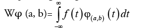
Consider a square-integrable, function f (t) then the continuous wavelet transform of f (t) corresponding to a given wavelet is
 (1)
(1)
where 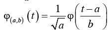 (2)
(2)
The function φ (t) is called the mother wavelet and by dilation and translation of φ (t) the wavelet φ(a,b)(t) is calculated. The terms a and b are called dilation and the translation factors respectively. There are different types of wavelets which are popular in feature extraction. The simple and much-preferred wavelet in feature extraction process is the Daubechies wavelet. DWT is the discrete version of equation(1) by confining a and b to a discrete lattice (a=2b & a>0). The expressions for DWT are:
 (3)
(3)
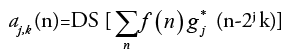
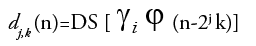
Equation (3) is considered as the fundamental equation for wavelet decomposition. In this decomposition process (FIGURE 2), the function f(n) is decomposed into the approximation coefficients a (n) and the detail components d (n). The wavelet scale and translation factors are represented by j and k, respectively. The down sampling is represented by the operator DS. The responses of low-pass and high-pass filters are represented by g (n) and h (n), respectively. This is called single-level decomposition and it can be repeated by decomposing the successive approximations continuously, to express a signal into different levels of resolution.

Figure 2: Decomposition process of 2D DWT.
■ 2D discrete wavelet transform
It is used to express the 2D images at various levels of resolution. Here the decomposition is done for each dimension independently. The following figure illustrates the decomposition process of the 2D image using DWT. At each scale it produces, 4 sub-band images named as LL, LH, HH and HL. The LL sub band is considered as the approximation coefficient of the image, while the LH, HL and HH sub bands are considered as the detailed components. Hence the LL sub-band is used for the next level of decomposition. As the decomposition level is increased, compact and coarser approximation coefficients can be achieved. In this algorithm, single level decomposition of Daubechies wavelet is used for the feature extraction.
■ Feature reduction
The high dimension feature vector increases the storage memory and computation time which leads to complicated and also misclassification. Hence the feature vector dimension has to be reduced. Principal Component Analysis (PCA) is the commonly used technique for the reduction of the feature vector. “It is the mean square optimal projection for Gaussian data leading to uncorrelated components by using second order statistics” [46]. But the higher order statistics are useful to capture the invariant features which are not considered by the PCA. The proposed method uses Independent Component analysis (ICA) for the reduction of the feature vector. ICA deals with higher order statistics and gives rise to independent components which can reveal interesting and fine features in the non-Gaussian hyper spectral image data sets. Hence ICA works more effectively than PCA in reducing the feature vector and also during the classification of brain tumors.
■ Independent component analysis (ICA)
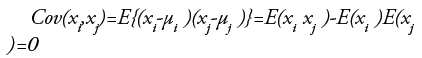
This topic is based on [47]. ICA is one of the higher-order methods. The projections of ICA are linear but not surely orthogonal. These are statistically independent to each other, which is a stronger condition than uncorrelated ness. The random variables x={x1,….xp} are said to be uncorrelated, if for ∀I ≠ j, 1 ≤ i, j≤p
In converse, the main requirement of
independent property is factorization of the
multivariate probability density function, which
can be written as 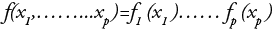
Independence property always entails
uncorrelated ness, but the vice versa is not there.
The two are equivalent only if the function  is multivariate
normal. Based on Fodor [47], the noise-free
ICA representation for a p-dimensional random
vector x follow to evaluate the components of
k-dimensional vector s and the p × k full column
rank matrix A
is multivariate
normal. Based on Fodor [47], the noise-free
ICA representation for a p-dimensional random
vector x follow to evaluate the components of
k-dimensional vector s and the p × k full column
rank matrix A
such that conferring to one of the definitions of independence the components of k-dimensional vector s is as independent as possible. "At least one of the hidden independent components si has to be non-Gaussian to ensure the identifiability of the model” [48]. This method uses 13 features like Mean, Standard-Deviation, Entropy, RMS, Variance, Smoothness, Kurtosis, Skewness, IDM, Contrast, Correlation, Energy and Homogeneity.
■ Classification using Kernel SVM
These are the extensions of linear SVMs and are nonlinear as these are using different nonlinear kernel functions. These KSVMs change the form of dot product in the SVMs which greatly reduces the number of dimension calculation. KSVMs have the various advantages [25,48]. 1. Less no. of tunable parameters; 2. It works very successfully in the fields categorization of natural language, computer vision and bioinformatics; 3. Training comprises of convex quadratic optimization which gives global and unique solutions, leading to the global minima convergence. It is the best advantage compared to neural networks. The reduced feature vector is submitted to KSVM to classify the tumor as benign or malignant. Four different kernels like linear, polynomial, RBF and quadratic are used for the evaluation and among them; quadratic kernel achieved the best classification accuracy.
■ Support vectors-hyper planes
Consider a few data points each point belongs to either of the two classes. Now the objective is how to classify a new data point. If the data point is a vector of p-dimension then a (p-1)- dimensional hyper plane is to be created. It may possible to have many hyper planes that can classify the data successfully but the one that exhibits largest gap or margin separating the two classes is considered as the best hyperplane since there should be a better classification for the new data during training. For this reason, the hyper plane is so chosen such that the gap between it and the closest point on both sides of it should be maximum [49]. FIGURE 3 represents the geometric interpolation of linear SVMs. Here the hyper planes H1, H2, H3 are used to classify the data points into two classes. The hyper plane H1 has a large margin to the support vectors S11, S12, S13, S21, S22 and S23, therefore it can do perfect classification [50]. But H2 and H3 can’t do the right classification as they do not have the largest margin.

Figure 3: The geometric interpolation of linear SVMs (H denotes for the hyper plane, S denotes for the support vector).
■ Principles of linear SVMs [25]
Consider a training dataset of size N and p-dimensional which is in the form

For class 1, yn is+1 and for class 2 it is -1 xn is a p-dimensional vector. To divide class 1 from class 2 hyper plane of maximum margin is needed. In general, hyper plane is in the form w.x-b=0 where w is the weight, a vector normal to the hyper plane and b is the bias and denotes the dot product.
The values of w and b are so chosen that they have to enlarge the gap between the two parallel hyper planes as wide as possible while still splitting the data as shown in FIGURE 4. The equation for two parallel hyper planes is w.x-b= ±1.

Figure 4: The parallel hyper planes.
The process of dividing the data is now an optimization problem, which involves the maximizing the margin between the two parallel hyper planes, by the condition of avoiding data falling into the margin.
■ Kernel support vector machinesa
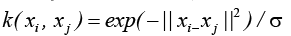
Linear SVMs uses a hyper plane to classify the data and these could not classify the data which is located at various sides of a hyper plane [25]. To overcome this problem kernel trick is used for SVMs [51]. This is similar to linear SVM, barring that the dot product is replaced by different nonlinear kernels. The equation of kernel is
with  which is in transformed
space. The dot products can be computed as
which is in transformed
space. The dot products can be computed as 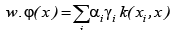 .Thus in a transformed
feature space KSVM allowed to fit the maximummargin
hyper plane and the classifier is a hyper
plane in the higher-dimensional feature space, it
may be non-linear in the original input space.
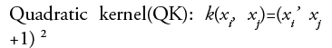
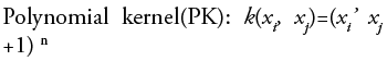
The proposed method uses four different kernels
like linear, polynomial, quadratic and radial
basis/Gaussian. The proposed four kernels are:
.Thus in a transformed
feature space KSVM allowed to fit the maximummargin
hyper plane and the classifier is a hyper
plane in the higher-dimensional feature space, it
may be non-linear in the original input space.
The proposed method uses four different kernels
like linear, polynomial, quadratic and radial
basis/Gaussian. The proposed four kernels are:
• Linear kernel(LK): 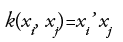
• 
• 
Radial Basis Function kernel(RBFK):
Evaluation
The efficiency of a segmentation algorithm is evaluated in two ways- subjective evaluation and objective evaluation. In the subjective evaluation the segmentation results are evaluated by human visualization which is a tedious process. The objective or automatic evaluation of segmentation is very easy and it involves verifying the segmented pixel against a known pixel-wise ground truth. There are mainly three performance parameters for any segmentation process, sensitivity, specificity and segmentation accuracy.
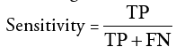
Sensitivity: It indicates true positivity and it is the probability that a detected or segmented pixel belongs to the tumor.
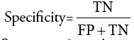
Specificity: It indicates true negativity and it is the probability that a detected or segmented pixel does not belong to the tumor but it belongs to the background.
Segmentation Accuracy: It indicates the degree to which a segmentation algorithm results matches with reference or ground truths.
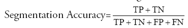
where TP indicates ‘True Positive’ which is the number of pixels exactly detected as tumor pixels.
TN indicates ‘True Negative’ which is the number of pixels exactly detected as not tumor pixels.
FP indicates ‘False Positive’ which is the number of pixels wrongly detected as tumor pixels.
FN indicates ‘False Negative’ which is the number of pixels wrongly detected as not tumor pixels.
Experimental Results and Discussion
The recommended ACM segmentation method is evaluated based on the above parameters and the performance of suggested method is compared with some of the previous methods like Otsu Binarization [25] and Fuzzy C-means [3] by applying different test MR images of the brain having benign and malignant tumors at various locations. The proposed method can be applied both on T1 and T2 weighted MR images. The results are very much similar if the images do not have any intensity inhomogeneity. The performance is estimated in the form of sensitivity, specificity, segmentation accuracy and classification accuracy.
FIGURES 5-14 demonstrates the segmentation results of 10 different MRI tumor Images for the proposed algorithm and the other methods like Otsu Binarization [18] and Fuzzy C-means [52]. The visual results demonstrate that proposed technique is great than the other. The segmentation accuracy of the current method is high which can increase the classification accuracy. This method performs well in segmentation as well as in classification compared to the previous methods. The evaluation of various SVM kernels is done in terms of their classification accuracy. The proposed Anisotropic+AC+DWT+ICA+KSVM with Gaussian or Radial Basis Function kernel method shows superiority to the linear, polynomial, quadratic kernel SVMs as its kernel is exponential, which can increase the distance between samples to a value than the other kernels.

Figure 5: Results of segmentation for test image 1: (a) Benign tumor image (T1- weighted) (b) ground truth (c). OTSU+DWT+PCA+KSVM results (d) FCM+DWT+ICA+KSVM results (e). Anisotropic+AC+DWT+ICA+KSVM results.

Figure 6: Results of segmentation for test image 2: (a) Benign tumor image (T1- weighted) (b) ground truth (c).OTSU+DWT+PCA+KSVM results (d) FCM+DWT+ICA+KSVM results (e) Anisotropic+AC+DWT+ICA+KSVM results.

Figure 7: Results of segmentation for test image 3: (a) Malignant tumor image (T2- weighted) (b) ground truth (c) OTSU+DWT+PCA+KSVM results (d) FCM+DWT+ICA+KSVM results (e) Anisotropic+AC+DWT+ICA+KSVM results.

Figure 8: Results of segmentation for test image 4: (a) Benign tumor image (T1- weighted) (b) ground truth (c) OTSU+DWT+PCA+KSVM results (d) FCM+DWT+ICA+KSVM results (e) Anisotropic+AC+DWT+ICA+KSVM results.

Figure 9: Results of segmentation for test image 5: (a) Malignant tumor image (T2- weighted) (b) ground truth (c) OTSU+DWT+PCA+KSVM results (d) FCM+DWT+ICA+KSVM results (e) Anisotropic+AC+DWT+ICA+KSVM results.

Figure 10: Results of segmentation for test image 6: (a) Benign tumor image (T2- weighted) (b) ground truth (c) OTSU+DWT+PCA+KSVM results (d) FCM+DWT+ICA+KSVM results (e) Anisotropic+AC+DWT+ICA+KSVM results.

Figure 11: Results of segmentation for test image 7: (a) Benign tumor image (T1- weighted) (b) ground truth (c) OTSU+DWT+PCA+KSVM results (d) FCM+DWT+ICA+KSVM results (e) Anisotropic+AC+DWT+ICA+KSVM results.

Figure 12: Results of segmentation for test image 8: (a) Malignant tumor image (T2- weighted) (b) ground truth (c) OTSU+DWT+PCA+KSVM results (d) FCM+DWT+ICA+KSVM results (e) Anisotropic+AC+DWT+ICA+KSVM results.

Figure 13: Results of segmentation for test image 9: (a) Malignant tumor image (T1- weighted) (b) ground truth (c) OTSU+DWT+PCA+KSVM results (d) FCM+DWT+ICA+KSVM results (e) Anisotropic+AC+DWT+ICA+KSVM results.

Figure 14: Results of segmentation for test image 10: (a) Malignant tumor image(T1-weighted) (b) groundtruth (c) OTSU+DWT+PCA+KSVM results (d) FCM+DWT+ICA+KSVM results (e) Anisotropic+AC+DWT+ICA+KSVM results.
TABLES 1-3 consists of the performance parameters of the proposed segmentation and classification algorithm-A n i s o t ropic+AC+DWT+ICA+KSVM (Anisotropic diffusion- filtering, ACsegmentation, DWT-feature extraction, PCAfeature reduction, KSVM-classification) and the existing methods OTSU+DWT+PCA+KSVM (OTSU-segmentation, DWT-feature extraction, PCA-feature reduction, KSVM-classification) [25], FCM [52]+DWT+ICA+KSVM (Fuzzy C-Means Clustering - segmentation, DWTfeature extraction, ICA-feature reduction, KSVM-classification) with different SVM kernels.
| Image | Sensitivity (%) | Specificity (%) | Segmentation Accuracy(%) | Classification Accuracy (%) | Type of tumor | |||
|---|---|---|---|---|---|---|---|---|
| RBF Kernel | Linear Kernel | polynomial Kernel | Quadratic Kernel | |||||
| 1 | 93.8642 | 96.3352 | 94.9325 | 70 | 70 | 60 | 60 | Benign |
| 2 | 92.8734 | 95.9549 | 94.7024 | 70 | 60 | 60 | 60 | Benign |
| 3 | 92.2512 | 95.3888 | 94.1169 | 80 | 70 | 60 | 70 | Malignant |
| 4 | 90.9779 | 96.1484 | 94.0056 | 70 | 60 | 70 | 70 | Benign |
| 5 | 94.7784 | 94.6694 | 95.7122 | 70 | 70 | 60 | 70 | Malignant |
| 6 | 92.5699 | 96.6992 | 97.0517 | 80 | 70 | 60 | 70 | Benign |
| 7 | 92.3755 | 97.6571 | 95.5137 | 80 | 70 | 70 | 70 | Benign |
| 8 | 92.4612 | 96.5707 | 94.8689 | 70 | 60 | 70 | 60 | Malignant |
| 9 | 92.1655 | 95.5765 | 93.7785 | 80 | 80 | 70 | 80 | Malignant |
| 10 | 92.2202 | 93.7002 | 94.8768 | 70 | 60 | 60 | 60 | Malignant |
Table 1: Performance measures of the OTSU+DWT+PCA+KSVM method.
| Image | Sensitivity (%) | Specificity (%) | Segmentation Accuracy (%) | Classification Accuracy (%) | Type of tumor | |||
|---|---|---|---|---|---|---|---|---|
| RBF Kernel | Linear Kernel | polynomial Kernel | Quadratic Kernel | |||||
| 1 | 94.7843 | 98.8552 | 96.1524 | 80 | 70 | 70 | 70 | Benign |
| 2 | 94.8758 | 97.2542 | 95.6324 | 80 | 70 | 70 | 70 | Benign |
| 3 | 96.5822 | 98.3698 | 97.5879 | 90 | 80 | 70 | 70 | Malignant |
| 4 | 93.3259 | 97.5879 | 96.5686 | 80 | 70 | 70 | 70 | Benign |
| 5 | 97.5694 | 97.4879 | 97.3256 | 80 | 70 | 70 | 70 | Malignant |
| 6 | 95.5369 | 97.4567 | 97.0345 | 90 | 80 | 70 | 70 | Benign |
| 7 | 94.3698 | 97.6235 | 96.9645 | 80 | 60 | 70 | 70 | Benign |
| 8 | 94.3698 | 96.5789 | 95.2356 | 80 | 70 | 60 | 70 | Malignant |
| 9 | 93.5655 | 97.8695 | 95.5698 | 90 | 80 | 80 | 80 | Malignant |
| 10 | 93.5902 | 94.5600 | 96.2786 | 80 | 70 | 70 | 70 | Malignant |
Table 2: Performance measures of the FCM+DWT+ICA+KSVM method.
| Image | Sensitivity (%) | Specificity (%) | Segmentation Accuracy (%) | Classification Accuracy (%) | Type of tumor | |||
|---|---|---|---|---|---|---|---|---|
| RBF Kernel | Linear Kernel | polynomial Kernel | Quadratic Kernel | |||||
| 1 | 95.8880 | 99.6379 | 98.3114 | 90 | 80 | 80 | 70 | Benign |
| 2 | 95.8966 | 99.3074 | 97.8152 | 90 | 80 | 80 | 80 | Benign |
| 3 | 97.2512 | 99.6888 | 99.1169 | 90 | 90 | 80 | 80 | Malignant |
| 4 | 94.9733 | 99.4415 | 97.3465 | 80 | 80 | 80 | 80 | Benign |
| 5 | 98.8080 | 99.7241 | 99.3645 | 90 | 80 | 80 | 80 | Malignant |
| 6 | 95.6269 | 99.8247 | 98.9504 | 100 | 90 | 80 | 90 | Benign |
| 7 | 94.4063 | 99.6775 | 97.9147 | 90 | 80 | 80 | 80 | Benign |
| 8 | 94.9706 | 99.7481 | 97.3555 | 90 | 80 | 80 | 80 | Malignant |
| 9 | 95.1232 | 98.7757 | 96.9640 | 90 | 80 | 90 | 80 | Malignant |
| 10 | 96.2024 | 99.8515 | 97.9428 | 90 | 80 | 80 | 80 | Malignant |
Table 3: Performance measures of the Anisotropic+AC+DWT+ICA+KSVM method.
This is a benign or low-grade tumor. Subjective or objective evaluation reveals that the proposed method is the best. When compared with ground truth, Images (c) and (d) consists of false positives which can decrease the specificity and segmentation accuracy.
This is also a benign tumor. Results reveal that the proposed method is the best. FCM result consists of false negatives which can decrease all the parameters sensitivity, specificity and segmentation accuracy. Otsu result consists of false positives which can decrease the specificity and segmentation accuracy.
This is a very complicated malignant tumor. It is considered as a high-grade tumor. OTSU and FCM are not able to identify the tumor part exactly, but our method did it very efficiently. OTSU and FCM results reveal that they consist of false positives and false negatives which can decrease all the parameters sensitivity, specificity and segmentation accuracy.
This is a benign tumor which is going to be converted into high-grade tumor very soon. Subjective or objective evaluation reveals that the suggested method is the best. The outcomes of the both OTSU and FCM are worst as these consist of many false positives and negatives which can decrease totally the performance of the algorithms.
This is a malignant tumor in its first stages. It is considered as high-grade tumor. OTSU and FCM are not able to identify the tumor part exactly, but our method did it very efficiently. OTSU and FCM results reveal that they consist of false positives and false negatives which can decrease all the parameters sensitivity, specificity and segmentation accuracy.
This is a simple benign tumor. Otsu results and FCM algorithms are results consists of false negatives and false positives which can decrease all the parameters sensitivity, specificity and segmentation accuracy.
This is a simple benign tumor. Otsu results and FCM algorithms are results consists of false negatives and false positives which can decrease all the parameters sensitivity, specificity and segmentation accuracy.
This is a complicated high-grade tumor which is very difficult to identify manually. Otsu and FCM algorithms are not able to identify exactly and segmented parts consist of false negatives and false positives which can decrease all the parameters like sensitivity, specificity and segmentation accuracy. The recommended method is able to identify it effectively compared to the previous two methods.
This is a highly effected brain with the tumor which is very difficult to identify manually. Otsu and FCM algorithms are not able to identify exactly and segmented parts consist of false negatives and false positives which can decrease all the segmentation performance parameters.
This is a malignant tumor image. Otsu and FCM algorithms are not able to identify exactly and segmented parts consist of false negatives and false positives which can decrease the performance of segmentation.
Conclusion
This paper proposed an innovative method to detect and to classify two different types of tumors in MRIs of the brain. This method outperforms well in segmentation as well as in classification. This method uses anisotropic diffusion filtering which are an excellent filtering technique for pre-processing and a more accurate Active Contour Model for the segmentation. To extract the features efficiently from the MR images of the tumor outstanding wavelet such as Daubechies wavelet is used.Independent Component analysis (ICA) is used to reduce the feature vector dimension. ICA deals with higher order statics to generate independent components revealing interesting and invariant features in the usually non-Gaussian hyper spectral data sets. Therefore ICA gives more meaningful results than PCA. As the brain MRI consists of nonlinear variations in the intensity of the pixels, linear SVMs are not preferred. Hence nonlinear Kernel SVMs are used for the classification of brain tumors. Kernels such as linear, polynomial, quadratic and GRB are considered. The results indicate that the GRB kernel achieved highest classification accuracy on all the test images than the other kernels. The reason of getting highest classification efficiency is its exponential form, which can elongate the space between samples to the degree that other kernels cannot do.
The performance of the proposed method can be enhanced for the purpose of diagnosis if it could be employed for all types of MRIs. Lift up wavelet transform can be used to decrease the computation time. Advanced kernels can be used to increase the classification accuracy. The excellent feature vector reduction methods such as manifold learning, KPCA, etc., can also be used. By Performing feature scaling and mean normalization for both test and train data and by increasing the number of features the classification efficiency can also be increased. With the proposed method tumors of any size can be detected provided proper contour is drawn.
There are writings illustrating Active contour models, wavelets, ICA, and SVMs. But this paper proposed a method that combines them as a powerful mechanism to identify tumors in MR images of the brain. This technique of brain tumor segmentation and classification based on Anisotropic, Active contour, Wavelet, ICA and KSVM is an efficient technique for the right treatment of the tumor.
References
- Demirhan A, Güler I. Image segmentation using self-organizing maps and gray level co-occurrence matrices. J. Fac. Eng. Arch. Gazi Univ. 25, 285-291 (2010).
- Chang HH, Valentino DJ, Duckwiler GR et al. Segmentation of brain MR images using a charged fluid model. IEEE. Trans. Biomed. Eng. 54, 1798-1813 (2007).
- Demirhan A, Törü M, Güler I. Segmentation of tumor and edema along with healthy tissues of brain using wavelets and neural networks. IEEE. J. Biomed. Health. Informatics. 19, 1451-1458 (2014).
- Ahmed S, Iftekharuddin KM, Vossough A. Efficacy of texture, shape, and intensity feature fusion for posterior-fossa tumor segmentation in MRI. IEEE. Trans. Inf. Technol. Biomed. 15, 206-213 (2011).
- Dou W, Ruan S, Chen Y et al. A framework of fuzzy information fusion for the segmentation of brain tumor tissues on MR images. Image. Vis. Comput. 25, 164-171 (2007).
- Zhang N, Ruan S, Lebonvallet S et al. Kernel feature selection to fuse multi-spectral MRI images for brain tumor segmentation. Comput. Vis. Image. Underst. 115, 256-269 (2011).
- Kaus MR, Warfield SK, Nabavi A et al. Automated segmentation of MR images of brain tumors. Radiology. 218, 586-591 (2001).
- Khotanlou H. 3D brain tumors and internal brain structures segmentation in MR images Ph.D. dissertation, Informatique, Telecommunications et Electronique, Telecom ParisTech, Paris. (2008).
- Kass M, Witkin A, Terzopoulos D. Snakes: active contour models. Int. J. Comput. Vis. 1, 321-331 (1988).
- Caselles V, Kimmel R, Sapiro G. Geodesic active contours. Processing of IEEE International Conference on Computer Vision, Boston, MA, pp. 694-699 (1995).
- Chan T, Vese L. Active contours without edges. IEEE. Trans. Image. Process. 10, 266-277 (2001).
- Zhu GP, Zhang ShQ, Zeng QSH et al. Boundary-based image segmentation using binary level set method. Opt. Eng. 46 (2007).
- Sandhya GK, Babu G, Satya Savithri T. Performance evaluation of active contours based methods for the detection of brain tumours in MR images. Int. J. Biomed. Eng. Technol. 18, 210-226 (2015).
- Gerig G, Kubler O, Kikinis R et al. Non-linear anisotropic filtering of MRI data. IEEE. Trans. Med. Imag. 11, 221-232 (1992).
- Mohamed FB, Vinitski S, Faro SH et al. Optimization of tissue segmentation of brain MR images based on multispectral 3D feature maps. Magnetic. Resonance. Imaging. 17, 403-409 (1999).
- Perona P, Malik J. Scale-space and edge detection using anisotropic diffusion. IEEE. Trans. Pattern. Anal. Mach. Intell. 12, 629-639 (1990).
- Iftekharuddin KM, Zheng J, Islam MA et al. Fractal-based brain tumor detection in multimodal MRI. Appl. Math. Comput. 207, 23-41 (2009).
- Zhou Z, Ruan Z. Multicontext wavelet-based thresholding segmentation of brain tissues in magnetic resonance images. Magnetic. Resonance. Imaging. 25, 381-385 (2007).
- Emin Tagluk M, Akin M, Sezgin N Classification of sleep apnea by using wavelet transform and artificial neural networks. Expert. Syst. Appl. 37, 1600-1607 (2010).
- Kwak N, Choi CH, Choi JY. Feature extraction using ICA ICANN. LNCS. 2130, 568-573 (2001).
- Wang J, Chang CI. Independent component analysis-based dimensionality reduction with applications in hyperspectral image analysis. IEEE. Trans. Geosci. Remote. Sens. 44 (2006).
- Lau PY, Voon FCT, Ozawa S. The detection and visualization of brain tumors on T2-weighted MRI images using multiparameter feature blocks. Int. Conf. Eng. Med. Biol. Soc. 5104-5107 (2006).
- Zhang Y, Wang S, Wu L. A novel method for magnetic resonance brain image classification based on adaptive chaotic progress in electromagnetics Research B Vol. 53, 2013 87 PSO. Prog. Electromagn. Res. 109, 325-343 (2010).
- Zhang Y, Wu L, Wang S. Magnetic resonance brain image classification by an improved artificial bee colony algorithm. Prog. Electromagn. Res. 116, 65-79 (2011).
- Zhang Y, Wu L. An MR brain images classifier via principal component analysis and kernel support vector machine. Prog. Electromagn. Res. 130, 369-388 (2012).
- El-Dahshan ES, Hosny T, Salem AM. Hybrid intelligent techniques for MRI brain images classification. Digital .Signal. Processing. 20, 433-441 (2010).
- Das S, Chowdhury M, Kundu MK. Brain MR image classification using multi-scale geometric analysis of ripplet. Prog. Electromagn. Res. 137, 1-17 (2013).
- Chaplot S, Patnaik LM, Jagannathan NR. Classification of magnetic resonance brain images using wavelets as input to support vector machine and neural network. Biomed. Signal. Process. Ctrl. 1, 86-92 (2006).
- Yeh JY, Fu JC. A hierarchical genetic algorithm for segmentation of multi-spectral human-brain MRI. Expert. Syst. Appl. 34, 1285-1295 (2008).
- Cocosco CA, Zijdenbos AP, Evans AC. A fully automatic and robust brain MRI tissue classification method. Med. Image. Anal. 7, 513-527 (2003).
- Patil NS, Shelokar PS, Jayaraman VK et al. Regression models using pattern search assisted least square support vector machines. Chem. Eng. Res. Des. 83, 1030-1037 (2005).
- Wang FF, Zhang YR. The support vector machine for dielectric target detection through a wall. Prog. Electromagn. Res. Lett. 23, 119-128 (2011).
- Xu Y, Guo Y, Xia L et al. An support vector regression based non-linear modeling method for Sic mesfet Prog. Electromagn. Res. Lett. 2, 103-114 (2008).
- Li D, Yang W, Wang S. Classification of foreign fibers in cotton lint using machine vision and multi-class support vector machine. Comput. Electron. Agric. 4, 274-279 (2010).
- Perona P, Malik J. Scale-space and edge detection using anisotropic diffusion. IEEE. Trans. Pattern Anal. Mach. Intell. 12, 629-639 (1990).
- Gerig G, Kubler O, Kikinis R et al. Non-linear anisotropic filtering of MRI data. IEEE. Trans. Med. Imag. 11, 221-232 (1992).
- Chan T, Vese L. Active contours without edges. IEEE. Trans. Image. Process. 10, 266-277 (2001).
- Cremers D, Rousson M, Deriche R. A review of statistical approaches to level set segmentation: integrating color, texture, motion and shape. Int. J. Comput. Vis. 72, 195-215 (2007).
- Ronfard R. Region-based strategies for active contour models. Int. J. Comput. Vis. 13, 229-251 (1994).
- Yezzi A, Tsai A, Willsky A. A statistical approach to snakes for bimodal and trimodal imagery, in: Seventh IEEE International Conference on Computer Vision, Washington, DC, USA. 2, 898-903 (1999).
- Samson C, Blanc-Feraud L, Aubert G et al. A variational model for image classification and restoration. IEEE. Trans. Pattern. Anal. Mach. Intell. 22, 460-472 (2000).
- Rousson M, Deriche R. A variational framework for active and adaptative segmentation of vector valued images. IEEE. Workshop. Motion. Video. Comput. 52-62 (2002).
- Wang Li, He L, Mishra A et al. Active contours driven by local Gaussian distribution fitting energy. Signal. Processing. 89, 2435-2447 (2009).
- Vaseghi S, Jetelova. H Principal and independent component analysis in image processing. Proceedings of the 14th ACM International Conference (2006).
- Fodor IK. A survey of dimension reduction techniques. Center for Applied Scientific Computing, Lawrence Livermore National Laboratory (2002).
- Bermejo S, Monegal B, Cabestany J. Fish age categorization from otolith images using multi-class support vector machines Fisheries. Research. 84, 247-253 (2007).
- Bishop CM. Pattern recognition and machine learning. Information Science and Statistics. Springer-Verlag. (2006).
- Vapnik V. The Nature of Statistical Learning Theory. Springer-Verlag. (1995).
- Acevedo-Rodriguez J, Maldonado-Bascón S, Lafuente-Arroyo S et al. Computational load reduction in decision functions using support vector machines. Signal. Processing. 89, 2066-2071 (2009).
- Balafar MA. Fuzzy C-mean based brain MRI segmentation algorithms. Springer-Artificial. Intelligence. Review. 41, 441-449 (2014).